Social Network Analysis in Python - Introduction to NetworkX

09 Sep 2019 - Written by Bartłomiej Czajewski

#python #networkx #social network analysis

background-picture

NetworkX is a Python library for working with graphs and perform analysis on them. It has built-in many fancy features like algorithms for creating specific graphs genres, or some centrality measures. But in this article we concentrate on work at grassroots - how to create graph, add and remove nodes and edges, add weighted edges, inspect graph properties an visualize graphs.

“By definition, a Graph is a collection of nodes (vertices) along with identified pairs of nodes (called edges, links, etc). In NetworkX, nodes can be any hashable object e.g., a text string, an image, an XML object, another Graph, a customized node object, etc.”
— NetworkX documentation

Content below is based on very good NetworkX documentation where you can go deeper into NetworkX. In this post you may see simple examples how to use code.

Contents:
1. Create a graph
2. Add nodes, edges, weighted edges to a graph
3. Add attributes to graphs, nodes, edges
4. Check a graph properties
5. Access edges and neighbors
6. Draw graphs
7. Graphs I/O in GML format

1. Create a graph

Create an empty graph

# Import library
import networkx as nx

# Create an empty graph - collection of nodes
G = nx.Graph()

# Create a directed graph using connections from the previous graph G
H = nx.DiGraph(G)

# Clear the graph from all nodes and edges 
# it deletes also graph attributes, nodes attributes and edges attributes.
G.clear()

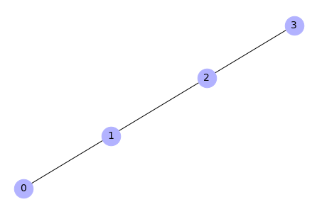
Create a graph from list of edges

# Create a list of edges (list of tuples)
edgelist = [(0, 1), (1, 2), (2, 3)]

# Create a graph
H = nx.Graph(edgelist)

# Draw a graph
%matplotlib inline

# Draw a plot
nx.draw(H, with_labels=True, node_color='#b2b2ff', node_size=700, 
	font_size=14)

Output:

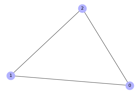
Create a graph from an adjacency matrix

# Create an adjacency matrix
import numpy as np
adj_m = np.array([[0, 1, 1],
                  [1, 1, 1],
                  [0, 1, 0]])

# Create a graph
G = nx.from_numpy_matrix(adj_m)

# Draw the graph
nx.draw(G, with_labels=True, node_color='#b2b2ff', node_size=700, 
	font_size=14)

Output:

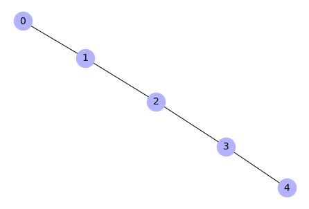
Create a chain graph

# Create a chain graph (5 nodes from 0 to 4)
H = nx.path_graph(5)

# Draw the graph
nx.draw(H, with_labels=True, node_color='#b2b2ff', node_size=700, 
	font_size=14)

Output:

2. Add nodes, edges, weighted edges to a graph

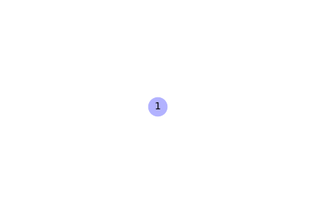
Add nodes to a graph

# Create an empty graph
G = nx.Graph()

# Add a node 
G.add_node(1)

# Draw the graph
nx.draw(G, with_labels=True, node_color='#b2b2ff', node_size=700, 
	font_size=14)

Output:

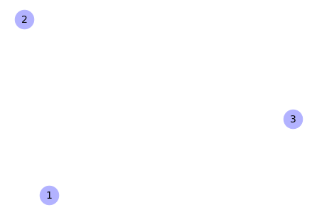
# Add a list of nodes
G.add_nodes_from([2, 3])

# Draw the graph
nx.draw(G, with_labels=True, node_color='#b2b2ff', node_size=700, 
	font_size=14)

Output:

# Create a chain graph (5 nodes from 0 to 4)
H = nx.path_graph(5)
# Show created nodes
H.nodes

Output:

NodeView((0, 1, 2, 3, 4))

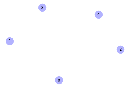
# Add nodes from the graph H to the graph G (nodes 1,2,3 are overwrited)
G.add_nodes_from(H)
G.nodes

Output:

NodeView((1, 2, 3, 0, 4))

We can see above that numbers play role of something like keys of particular nodes in graph. And this nodes may be overwritten.

# Draw the graph
nx.draw(G, with_labels=True, node_color='#b2b2ff', node_size=700, 
	font_size=14)

Output:

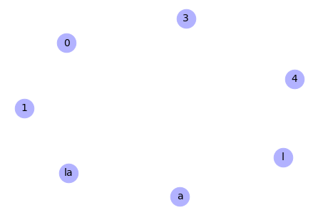
# Add a node as a string label
G.add_node("la") # adds node "la"
G.nodes

Output:

NodeView((1, 2, 3, 0, 4, 'la'))

# Add nodes as single string elements
G.add_nodes_from("la")  # adds 2 nodes: 'l', 'a'
G.nodes

Output:

NodeView((1, 2, 3, 0, 4, 'la', 'l', 'a'))

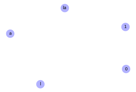
Remove nodes from the graph

# Remove a node
G.remove_node(2)

# Draw the graph
nx.draw(G, with_labels=True, node_color='#b2b2ff', node_size=700, 
	font_size=14)

Output:

# Remove nodes from an iterable container
G.remove_nodes_from([3,4])

# Draw the graph
nx.draw(G, with_labels=True, node_color='#b2b2ff', node_size=700, 
	font_size=14)

Output:

Add edges to a graph

# Create an empty graph
G = nx.Graph()

# Add an edge between node 1 and node 2
G.add_edge(1, 2)

# Draw the graph
nx.draw(G, with_labels=True, node_color='#b2b2ff', node_size=700, 
	font_size=14)

Output:

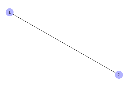
We can see above that if an edge is created - all needed non-existing nodes are created as well.

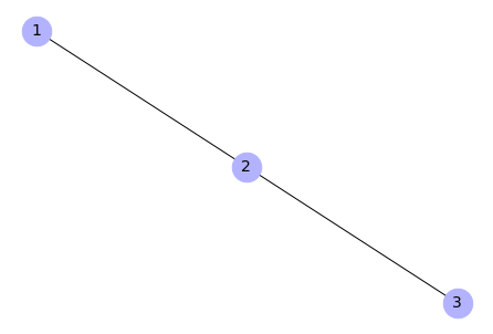
# Create a tuple with 2, 3
e = (2, 3)
type(e)

Output:

tuple

# Use the tuple to create an edge between nodes 2 and 3
G.add_edge(*e)
G.edges

Output:

EdgeView([(1, 2), (2, 3)])

# Draw the graph
nx.draw(G, with_labels=True, node_color='#b2b2ff', node_size=700, 
	font_size=14)

Output:

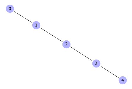
# Create a chain graph (5 nodes from 0 to 4)
H = nx.path_graph(5)
# Add edges to graph G from graph H
G.add_edges_from(H.edges)
G.edges

Output:

EdgeView([(1, 2), (1, 0), (2, 3), (3, 4)])

# Draw the graph
nx.draw(G, with_labels=True, node_color='#b2b2ff', node_size=700, 
	font_size=14)

Output:

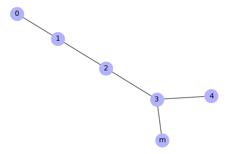
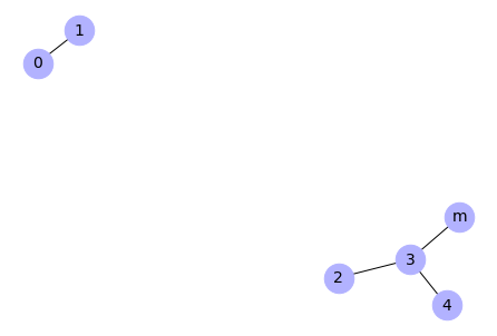
# Add an edge between node 3 and non-existing node m - which is automatically
#                                                                  created
G.add_edge(3, 'm')

# Draw the graph
nx.draw(G, with_labels=True, node_color='#b2b2ff', node_size=700, 
	font_size=14)

Output:

Remove edges from a graph

# Remove an edge
G.remove_edge(1, 2)

# Draw the graph
nx.draw(G, with_labels=True, node_color='#b2b2ff', node_size=700, 
	font_size=14)

Output:

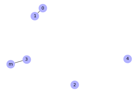
# Remove edges from an iterable container
G.remove_edges_from([(2, 3),(3,4)])

# Draw the graph
nx.draw(G, with_labels=True, node_color='#b2b2ff', node_size=700, 
	font_size=14)

Output:

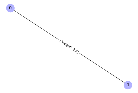
Add weighted edges to a graph

# Create an empty graph
G = nx.Graph()

# Add an edge with weight as a tuple with a dictionary inside on a 3rd position  
G.add_edge(0, 1, weight=2.8)

G.edges

Output:

EdgeView([(0, 1)])

# Compute a position of the graph elements (needed to visualize weighted graphs)
pos = nx.spring_layout(G)
# Draw the graph
nx.draw(G, pos = pos, with_labels=True, node_color='#b2b2ff', node_size=700, 
	font_size=14)
# Add weights to the graph picture
nx.draw_networkx_edge_labels(G, pos)

Output:

{(0, 1): Text(0.0, 0.0, "{'weight': 2.8}")}

Output:

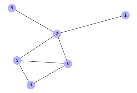
Create Erdős-Rényi graph

For an example we use Erdős-Rényi graph generation. It takes only one short line of code. This is a simple and powerful way of creating graphs. Method “erdos_renyi_graph()” takes 2 arguments. 1st is number of nodes, and second one is probability that a node will get an edge connection with every other particular node. So if more nodes, probability of node having any edge rise.

# Import library
import random
import numpy as np

# Generate Erdos-renyi graph 
G = nx.gnp_random_graph(6,0.4) # (gnp alias from: G-raph, N-odes, 
                               #                    P-robability)
nx.draw(G, with_labels=True, node_color='#b2b2ff', node_size=700, 
	font_size=14)

Output:

Add random weights to the graph

# add random weights 
for u,v,d in G.edges(data=True):
    d['weight'] = round(random.random(),2) # there we may set distribution
    # in this loop we iterate over a tuples in a list
    #                    u - is actually 1st node of an edge
    #                    v - is second node of an edge
    #                    d - is dict with weight of edge

# Extract tuples of adges, and weights from the graph
edges,weights = zip(*nx.get_edge_attributes(G,'weight').items())
print(weights, edges)

# Compute a position of graph elements (needed to visualize weighted graphs)
pos = nx.spring_layout(G)
# draw graph
nx.draw(G, pos = pos, with_labels=True, node_color='#b2b2ff', node_size=700, 
	font_size=14)
# Add weights to graph picture
nx.draw_networkx_edge_labels(G, pos)

Output:

(0.67, 0.28, 0.31, 0.61, 0.66, 0.13, 0.63) ((0, 2), (0, 4), (0, 5), (1, 2), (2, 3), (2, 5), (4, 5))

Output:

{(0, 2): Text(0.05587924164442272, 0.03572413385076614, "{'weight': 0.67}"),
 (0, 4): Text(-0.09144909073877293, -0.6331454386897136, "{'weight': 0.28}"),
 (0, 5): Text(-0.18708205101864206, -0.43166771273736326, "{'weight': 0.31}"),
 (1, 2): Text(0.36606551732176823, 0.4975472153877831, "{'weight': 0.61}"),
 (2, 3): Text(-0.03165513391993038, 0.6029900698900599, "{'weight': 0.66}"),
 (2, 5): Text(-0.14019660265009343, -0.12965270150716987, "{'weight': 0.13}"),
 (4, 5): Text(-0.2875249350332891, -0.7985222740476496, "{'weight': 0.63}")}

Output:

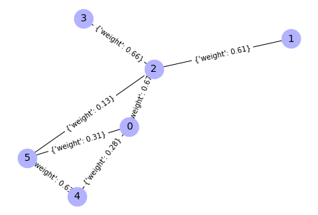
Note that positions of nodes may differ from the unweighted graph, but structure of the graph is the same

3. Add attributes to a graph, nodes and edges

Add attributes to a graph

# Create a graph
G = nx.Graph()
# Add 'day' attribute to the graph with "Friday" value
G = nx.Graph(day = "Friday")
G.graph

Output:

{'day': 'Friday'}

# Change an attribute value
G.graph['day'] = "Monday"
G.graph

Output:

{'day': 'Monday'}

# Delete graph attribute
del G.graph['day']

G.graph

Output:

{}

Add attributes to nodes

# Create a graph
G = nx.Graph()

# Add an attribute "time" with value, for node 1
G.add_node(1, time='5pm')

# Add the attribute "time" with value, for node 3
G.add_nodes_from([3], time='2pm')

# Check attributes of 1 node
G.nodes[1]

Output:

{'time': '5pm'}

# Check attributes of 3 node
G.nodes[3]

Output:

{'time': '2pm'}

# Add an attribute "room" with value, for node 1
G.nodes[1]['room'] = 714
G.nodes.data()

Output:

NodeDataView({1: {'time': '5pm', 'room': 714}, 3: {'time': '2pm'}})

# delete particular node attribute
del G.nodes[1]['room']

# Print nodes attributes
G.nodes.data()

Output:

NodeDataView({1: {'time': '5pm'}, 3: {'time': '2pm'}})

# Print nodes attributes
for k, v in G.nodes.items():
    print(f'{k:<4} {v}')

Output:

1    {'time': '5pm'}
3    {'time': '2pm'}

# Delete 'time' attributes from all nodes in a loop
for k, v in G.nodes.items():
    del G.nodes[k]['time']

# Print node attributes
for k, v in G.nodes.items():
    print(f'{k:<4} {v}')

Output:

1    {}
3    {}

Add attributes to an edges

# Create a graph
G = nx.Graph()

# Add weighted edge to graph    
G.add_edge(1, 2, weight=4.7 )

# Compute position of the graph elements
pos = nx.spring_layout(G)
# Draw the graph
nx.draw(G, pos = pos, with_labels=True, node_color='#b2b2ff', node_size=700, 
	font_size=14)
# Add weights to a graph picture
nx.draw_networkx_edge_labels(G, pos)

Output:

{(1, 2): Text(2.220446049250313e-16, 0.0, "{'weight': 4.7}")}

Output:

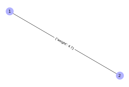
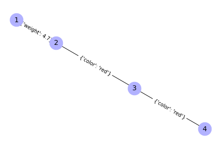
Weights are one type of attributes. We may create custom attributes.

# Add 2 edges with attribute color to the graph     
G.add_edges_from([(2, 3), (3, 4)], color='red')

# Compute a position of graph elements
pos = nx.spring_layout(G)
# Draw the graph
nx.draw(G, pos = pos, with_labels=True, node_color='#b2b2ff', node_size=700, 
	font_size=14)
# Add attributes to graph picture
nx.draw_networkx_edge_labels(G, pos)

Output:

{(1, 2): Text(-0.6545391148791944, 0.17485675574125337, "{'weight': 4.7}"),
 (2, 3): Text(-0.07544906355289227, 0.020149585725262716, "{'color': 'red'}"),
 (3, 4): Text(0.6545391148791944, -0.17485675574125328, "{'color': 'red'}")}

Output:

# Another way to add an attribute
G.add_edges_from([(1, 2, {'color': 'blue'}), (2, 3, {'weight': 8})])

# Another way to add an attribute
G.edges[1,2]['color'] = "white"
# Check added properties of edges
G.adj.items()

Output:

ItemsView(AdjacencyView({1: {2: {'weight': 4.7, 'color': 'white'}}, 2: {1: {'weight': 4.7, 'color': 'white'}, 3: {'color': 'red', 'weight': 8}}, 3: {2: {'color': 'red', 'weight': 8}, 4: {'color': 'red'}}, 4: {3: {'color': 'red'}}}))

# Print edges attributes in more readable way 
for k, v, w in G.edges.data():
    print(f'{k:<4} {v}{w}')

Output:

  2{'weight': 4.7, 'color': 'white'}
  3{'color': 'red', 'weight': 8}
  4{'color': 'red'}

In the printings above we can see that node 1 has connection with node 2. And this edge has attributes weight and color. Node 2 has 2 connections - with node 1 and node 3.

# Add a weight for an edge 1-2
G[1][2]['weight'] = 4.7

# or
G.edges[1, 2]['weight'] = 4.7    

# Check attributes on edges
G.edges.data()

Output:

EdgeDataView([(1, 2, {'weight': 4.7, 'color': 'white'}), (2, 3, {'color': 'red', 'weight': 8}), (3, 4, {'color': 'red'})])

# Print edges attributes in more readable way 
for k, v, w in G.edges.data():
    print(f'{k:<4} {v}{w}')

Output:

  2{'weight': 4.7, 'color': 'white'}
  3{'color': 'red', 'weight': 8}
  4{'color': 'red'}

# Delete edge attribute 
del G[2][3]['color']

# Print edges attributes 
for k, v, w in G.edges.data():
    print(f'{k:<4} {v}{w}')

Output:

  2{'weight': 4.7, 'color': 'white'}
  3{'weight': 8}
  4{'color': 'red'}

G.edges.data()

Output:

EdgeDataView([(1, 2, {'weight': 4.7, 'color': 'white'}), (2, 3, {'weight': 8}), (3, 4, {'color': 'red'})])

# Delete edge attributes "weight"
for n1, n2, d in G.edges(data=True):
    if "weight" in d:
        del d["weight"]

# Print edges attributes 
for k, v, w in G.edges.data():
    print(f'{k:<4} {v}{w}')

Output:

  2{'color': 'white'}
  3{}
  4{'color': 'red'}

4. Check a graph properties

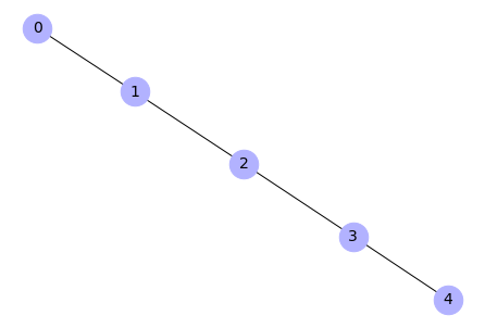
Prepare a graph

# Create a chain graph
G = nx.path_graph(5)
# Draw the graph
nx.draw(G, with_labels=True, node_color='#b2b2ff', node_size=700, 
	font_size=14)

Output:

Check properties

# Check number of nodes
G.number_of_nodes()

Output:

# Check number of edges
G.number_of_edges()

Output:

Nodes View

# All nodes overview
G.nodes()

Output:

NodeView((0, 1, 2, 3, 4))

# or
list(G.nodes)

Output:

[0, 1, 2, 3, 4]

# or
G.nodes.items()

Output:

ItemsView(NodeView((0, 1, 2, 3, 4)))

# or
G.nodes.data()

Output:

NodeDataView({0: {}, 1: {}, 2: {}, 3: {}, 4: {}})

# or
G.nodes.data('span')

Output:

NodeDataView({0: None, 1: None, 2: None, 3: None, 4: None}, data='span')

Edges View

# All edges overview
G.edges

Output:

EdgeView([(0, 1), (1, 2), (2, 3), (3, 4)])

# or
list(G.edges)

Output:

[(0, 1), (1, 2), (2, 3), (3, 4)]

# or
G.edges.items()

Output:

ItemsView(EdgeView([(0, 1), (1, 2), (2, 3), (3, 4)]))

# or (weights visible)
G.edges.data()

Output:

EdgeDataView([(0, 1, {}), (1, 2, {}), (2, 3, {}), (3, 4, {})])

# or (weights visible)
G.edges.data('span')

Output:

EdgeDataView([(0, 1, None), (1, 2, None), (2, 3, None), (3, 4, None)])

# or (for an iterable container of nodes) - all edges associated with this 
#                                                       subset of nodes
G.edges([2, 'm'])

Output:

EdgeDataView([(2, 1), (2, 3)])

Node degree View

# Check degree of particular nodes
G.degree

Output:

DegreeView({0: 1, 1: 2, 2: 2, 3: 2, 4: 1})

# list degrees in column (":<4" makes 4 spaces between numbers)
for v, d in G.degree():
    print(f'{v:<4} {d}')

Output:

# or (for the one particular node)
G.degree[1]

Output:

# or (for the iterable container of nodes)
G.degree([2, 3])

Output:

DegreeView({2: 2, 3: 2})

Adjacency view

# Check an adjacency matrix - neighbourhood between nodes
G.adj

Output:

AdjacencyView({0: {1: {}}, 1: {0: {}, 2: {}}, 2: {1: {}, 3: {}}, 3: {2: {}, 4: {}}, 4: {3: {}}})

# Print a dictionary in a dictionary in more readable way 
from pprint import pprint
pprint(dict(G.adj))

Output:

{0: AtlasView({1: {}}),
AtlasView({0: {}, 2: {}}),
AtlasView({1: {}, 3: {}}),
AtlasView({2: {}, 4: {}}),
AtlasView({3: {}})}

# Check neighbors of particular node
list(G.adj[3])

Output:

[2, 4]

# or
G[3]

Output:

AtlasView({2: {}, 4: {}})

# or
list(G.neighbors(3))

Output:

[2, 4]

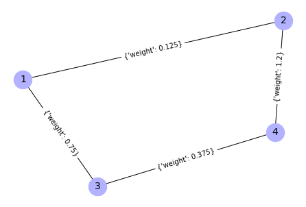
5. Accessing edges and neighbors

# Create a graph
G = nx.Graph()
G.add_weighted_edges_from([(1, 2, 0.125), (1, 3, 0.75), (2, 4, 1.2), 
                           (3, 4, 0.375)])

# Compute position of graph elements
pos = nx.spring_layout(G)
# Draw the graph
nx.draw(G, pos = pos, with_labels=True, node_color='#b2b2ff', node_size=700, 
	font_size=14)
# Add weights to a graph picture
nx.draw_networkx_edge_labels(G, pos)

Output:

{(1, 2): Text(-0.11306457583748142, 0.3689242447964494, "{'weight': 0.125}"),
 (1, 3): Text(-0.7453632597697203, -0.1911266592810591, "{'weight': 0.75}"),
 (2, 4): Text(0.74536325976972, 0.19112665928105907, "{'weight': 1.2}"),
 (3, 4): Text(0.11306457583748117, -0.3689242447964495, "{'weight': 0.375}")}

Output:

1st method for edges + weights extraction

# Get 'weight' attributes
nx.get_edge_attributes(G,'weight').items()

Output:

dict_items([((1, 2), 0.125), ((1, 3), 0.75), ((2, 4), 1.2), ((3, 4), 0.375)])

# Build up variables
edges,weights = zip(*nx.get_edge_attributes(G,'weight').items())

# Edges overview
edges # tuple of tuples

Output:

((1, 2), (1, 3), (2, 4), (3, 4))

# Weights overview
weights # tuple

Output:

(0.125, 0.75, 1.2, 0.375)

2nd method for edges + weights extraction

for (u, v, wt) in G.edges.data('weight'):
    print('(%d, %d, %.3f)' % (u, v, wt))

Output:

(1, 2, 0.125)
(1, 3, 0.750)
(2, 4, 1.200)
(3, 4, 0.375)

2nd method for edges + weights extraction with condition

for (u, v, wt) in G.edges.data('weight'):
    if wt < 0.5: print('(%d, %d, %.3f)' % (u, v, wt))

Output:

(1, 2, 0.125)
(3, 4, 0.375)

6. Draw graphs

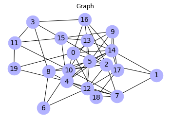
Figure size changing

# Import libraries
import networkx as nx
import matplotlib.pyplot as plt

# Graph creation
G = nx.erdos_renyi_graph(20, 0.30)

# Draw a graph
plt.figure(1) # default figure size 
plt.title("Graph") # Add title
nx.draw(G, with_labels=True, node_color='#b2b2ff', node_size=700, 
	font_size=14)

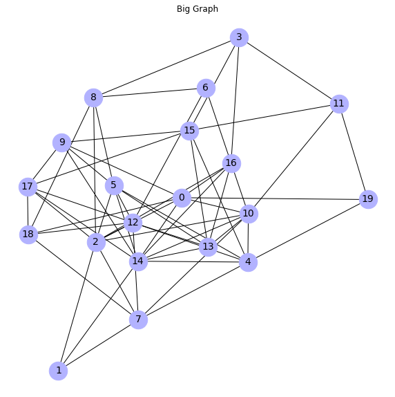
# Draw a big graph
plt.figure(2,figsize=(10,10)) # Custom figure size
plt.title("Big Graph") # Add title
nx.draw(G, with_labels=True, node_color='#b2b2ff', node_size=700, 
	font_size=14)

Output:

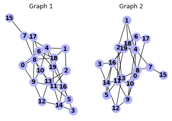
Draw 2 graphs on 1 chart

# Create graph
G = nx.erdos_renyi_graph(20, 0.20)

# Draw graphs with "nx.draw" and subplots 
# Nr 121, 122 are for 2 graphs on 1 chartplt.subplot(121)

# Draw graph 1
plt.subplot(121)
plt.title("Graph 1")
nx.draw(G, with_labels=True, node_color='#b2b2ff', node_size=700, 
	font_size=14)

# Draw graph 2
plt.subplot(122)
plt.title("Graph 2")
nx.draw(G, with_labels=True, node_color='#b2b2ff', node_size=700, 
	font_size=14)

Output:

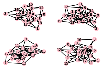
Draw 4 graphs on 1 chart with kwargs

In the situation where we have to define arguments for many subplots we may use “kwargs” (keyworded arguments) feature. It allows us to define a dictionary contains keys with values, which become arguments of a function. Clear explanation of this feature you may find there.

# Create graph
G = nx.erdos_renyi_graph(20, 0.30)

# Define **kwargs - dictionary with arguments for a function
kwargs = {
    'node_color': 'pink',
    'node_size': 200,
    'width': 2, # 
    }

# Draw graphs with options
# Nr 221, 222, 223, 224 are for 4 graphs on 1 chart
plt.subplot(221)
nx.draw(G, with_labels=True, font_weight='bold', **kwargs)
plt.subplot(222)
nx.draw(G, with_labels=True, font_weight='bold', **kwargs)
plt.subplot(223)
nx.draw(G, with_labels=True, **kwargs)
plt.subplot(224)
nx.draw(G, with_labels=True, **kwargs)

Output:

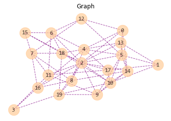
Draw a graph with more arguments specified

plt.title("Graph")
nx.draw(G, # graph object 
        with_labels=True, # label of node (numbers of nodes in this case)
        node_size=500, 
        node_color="#ffcc99", 
        node_shape="o", 
        alpha=0.7, # node transparency
        linewidths=1, # linewidth of symbol borders (nodes)
        width=1, # linewidth of edges
        edge_color="purple", 
        style="dashed", # style of edges
        font_size=12, 
        fontcolor="k", 
        font_family="Consolas")

Output:

with_labels (bool, optional (default=True)) – Set to True to draw labels on the nodes.
node_size (scalar or array, optional (default=300)) – Size of nodes. If an array is specified it must be the same length as nodelist
node_color (color string, or array of floats, (default=’#1f78b4’)) – Node color. Can be a single color format string, or a sequence of colors with the same length as nodelist. If numeric values are specified they will be mapped to colors using the cmap and vmin,vmax parameters. See matplotlib.scatter for more details.
node_shape (string, optional (default=’o’)) – The shape of the node. Specification is as matplotlib.scatter marker, one of ‘so^>v<dph8’.
alpha (float, optional (default=1.0)) – The node and edge transparency
linewidths ([None | scalar | sequence]) – Line width of symbol border (default =1.0)
width (float, optional (default=1.0)) – Line width of edges
edge_color (color string, or array of floats (default=’r’)) – Edge color. Can be a single color format string, or a sequence of colors with the same length as edgelist. If numeric values are specified they will be mapped to colors using the edge_cmap and edge_vmin,edge_vmax parameters.
style (string, optional (default=’solid’)) – Edge line style (solid|dashed|dotted,dashdot)
font_size (int, optional (default=12)) – Font size for text labels
font_color (string, optional (default=’k’ black)) – Font color string
font_family (string, optional (default=’sans-serif’)) – Font family

Check more arguments in NetworkX documentation.

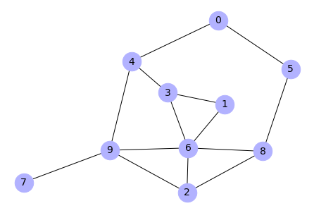
Add random weights to a graph and draw as colored edges

Very interesting way for visualize weighted graph is to color its edges depending on weights.

# Generate Erdős-Rényi graph
G = nx.gnp_random_graph(10,0.3)
nx.draw(G, with_labels=True, node_color='#b2b2ff', node_size=700, 
	font_size=14)

Output:

# Add random weights 
for u,v,d in G.edges(data=True):
    d['weight'] = random.random() # there we may set distribution
    # in this loop we iterate over a tuples in a list
    #                    u - is actually 1st node of an edge
    #                    v - is second node of an edge
    #                    d - is dict with weight of edge
    
# Extract tuples of adges, and weights from the graph
edges,weights = zip(*nx.get_edge_attributes(G,'weight').items())

# Compute optimized nodes positions
pos = nx.spring_layout(G)
# Draw graph
nx.draw(G, pos, edgelist=edges, 
        edge_color=weights, width=3.0, edge_cmap=plt.cm.Blues, 
        edge_vmin=-0.4, edge_vmax=1, with_labels=True,
		node_color='#b2b2ff', node_size=700, font_size=14)

Output:

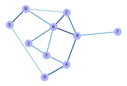
Note that positions of nodes may differ from the unweighted graph, but structure of the graph is the same.

7. Graphs I/O in GML format

write GML file nx.write_gml(graph, "path.to.file")
read GML file mygraph = nx.read_gml("path.to.file")

Annotation

Instructions are dedicated for Windows 10
Anaconda release: 2019.03
Python version: 3.7.3
networkx==2.3

Everyday normal hacker data science and coding

Social Network Analysis in Python - Introduction to NetworkX

1. Create a graph

Create an empty graph

Create a graph from list of edges

Create a graph from an adjacency matrix

Create a chain graph

2. Add nodes, edges, weighted edges to a graph

Add nodes to a graph

Remove nodes from the graph

Add edges to a graph

Remove edges from a graph

Add weighted edges to a graph

Create Erdős-Rényi graph

Add random weights to the graph

3. Add attributes to a graph, nodes and edges

Add attributes to a graph

Add attributes to nodes

Add attributes to an edges

4. Check a graph properties

Prepare a graph

Check properties

Nodes View

Edges View

Node degree View

Adjacency view

5. Accessing edges and neighbors

1st method for edges + weights extraction

2nd method for edges + weights extraction

2nd method for edges + weights extraction with condition

6. Draw graphs

Figure size changing

Draw 2 graphs on 1 chart

Draw 4 graphs on 1 chart with kwargs

Draw a graph with more arguments specified

Add random weights to a graph and draw as colored edges

7. Graphs I/O in GML format

Annotation

Related Posts