DifPy - Diffusion on Graphs in Python [PL]

#python   #difpy   #multi-agent modelling   #diffusion   #social network analysis

W niniejszym artykule chciałbym przedstawić DifPy - pakiet do symulacji wieloagentowych napisany w języku Python, który jest obecnie na wczesnym etapie rozwoju. Główne funkcjonalności pakietu to tworzenie grafów do symulacji, przeprowadzanie symulacji wieloagentowych na grafach, wybór zestawu wierzchołków, które najlepiej rozprowadzają informacje po grafie, oraz badanie związku statystycznego cech przypisanych do węzłów, ze zdolnością tych węzłów do propagacji informacji. Kod źródłowy wraz ze wskazówkami dotyczącymi instalacji opublikowano w serwisie GitHub na licencji MIT - DifPy repository.

Pakiet DifPy składa się z 12 funkcji zawartych w 4 modułach - module inicjalizującym, symulacyjnym, optymalizacyjnym i modelująco-objaśniającym. Napisano pięć funkcji modułu inicjalizującego służących do tworzenia i modyfikowania grafów, obliczania ich podstawowych charakterystyk i wizualizacji. Moduł symulacyjny składa się z trzech funkcji, które umożliwiają przeprowadzanie symulacji wieloagentowych na grafach. Do obliczania zdolności węzłów do propagacji informacji wykorzystywana jest metoda Monte Carlo. Moduł optymalizacyjny jest odpowiedzialny za typowanie zadanego n najlepszych wierzchołków w danej sieci, które możliwie najlepiej rozpropagują informację. Zaprojektowano dwie funkcje – jedną wyznaczającą n wierzchołków na podstawie miary centralności – bliskości (ang. closeness), oraz drugą funkcję realizującą te samą funkcjonalność symulacyjnie za pomocą metody Monte Carlo i losowego przeszukiwania przestrzeni rozwiązań. W Module modelująco-objaśniającym zaimplementowano funkcjonalność identyfikacji cech jednostek w danej sieci społecznej, które najlepiej rozpropagują informację, lub wypromują produkt. Funkcjonalności tej odpowiadają dwie funkcje. Pierwsza z nich oblicza zdolność wierzchołków grafu do rozprowadzania informacji. Druga z nich wykorzystuje funkcję pierwszą – oblicza miary wierzchołków, zestawia je z cechami węzłów, tworzy model xgboost, a następnie oblicza istotność badanych cech.

Pakiet DifPy napisano z myślą o przeprowadzaniu eksperymentów na grafach reprezentujących rzeczywiste sieci społeczne. Prowadzenie eksperymentów symulacyjnych może wymagać odwzorowania danych o sieci, którymi dysponujemy, w graf biblioteki NetworkX. Artykuł o podstawach pracy z tą biblioteką można znaleźć tutaj - Social Network Analysis in Python - Introduction to NetworkX.

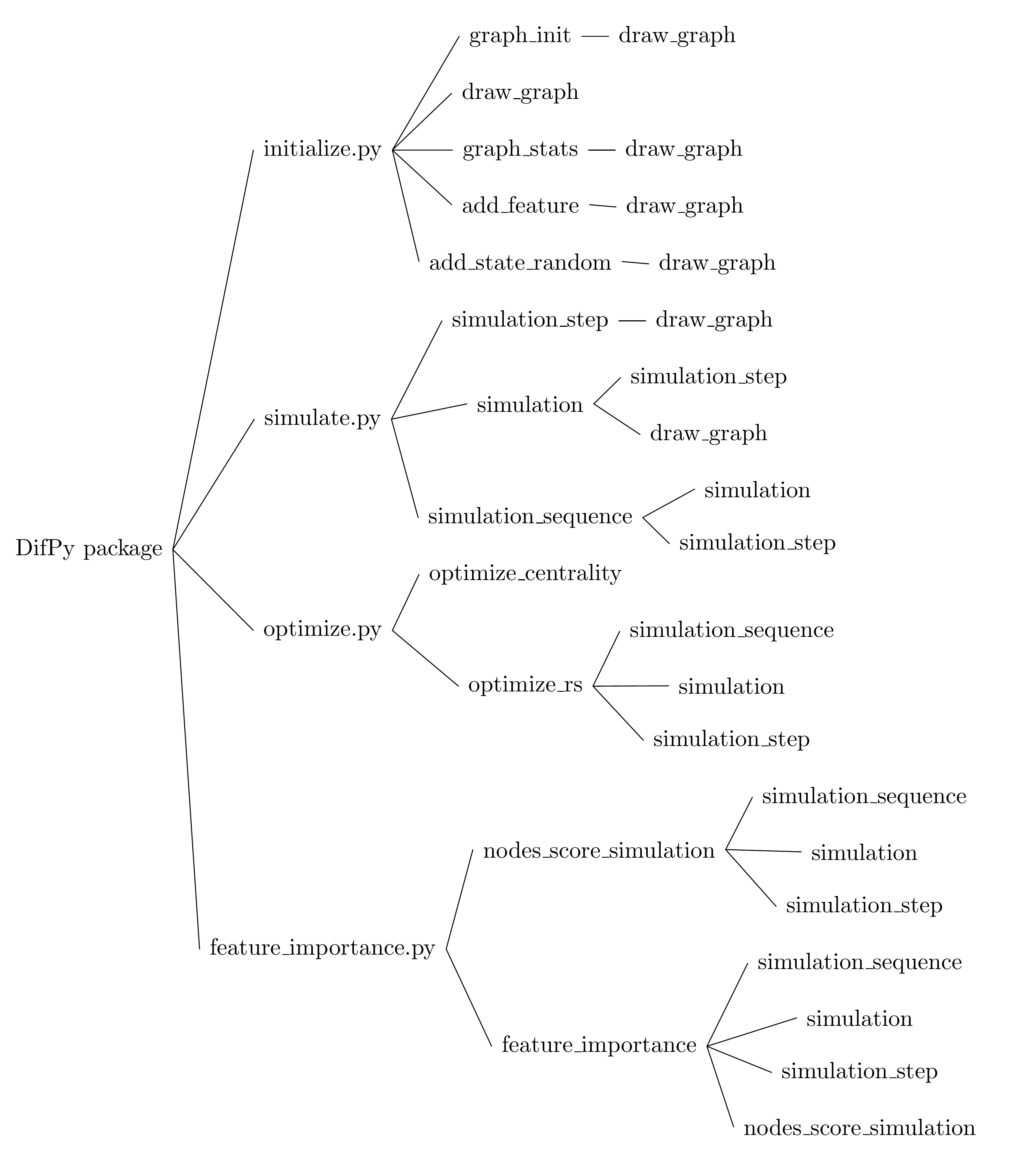
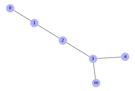
Rysunek 1. Struktura pakietu DifPy

Powyższy rysunek przedstawia strukturę pakietu DifPy rozpisaną na poszczególne moduły, funkcje i zależności tych funkcji. Korzeń drzewa reprezentuje pakiet DifPy. Węzły na pierwszym poziomie odzwierciedlają moduły pakietu. Węzły na trzecim poziomie oznaczają funkcje, natomiast czwarty poziom odnosi się do funkcji, które są wywoływane przez funkcje na trzecim stopniu drzewa.

Poniżej importowana jest biblioteka DifPy. Podczas uruchamiania jej funkcji automatycznie odnosi się ona do innych bibliotek takich jak NetworkX, czy Numpy, więc nie ma potrzeby ich dodatkowego importowania.

import difpy as dp

W dalszej części artykułu zaprezentowano działanie funkcji pakietu DifPy. Dane do przykładów generowane są w sposób losowy z wykorzystaniem modułu initialize.py, opierając się na mechanizmach losowego generowania sieci i cech zaczerpniętych z bibliotek NetworkX i Numpy. Ponadto do przetestowania funkcji z czwartego modułu badającej istotność cech, wygenerowano losowe zmienne z wykorzystaniem bibliotek Numpy, SciPy, math oraz statsmodels.

Contents:
1. Moduł inicjalizujący
2. Moduł symulacyjny
3. Moduł optymalizacyjny
4. Moduł modelująco-wyjaśniający

1. Moduł inicjalizujący

Moduł inicjalizujący initialize.py utworzono w celu ułatwienia generowania grafów i dostosowywania istniejących już grafów do przeprowadzenia symulacji.

Moduł inicjalizujący zawiera pięć funkcji. Funkcja graph_init() służy do utworzenia przykładowego grafu gotowego do przeprowadzenia symulacji. Funkcja draw_graph() jest funkcją pomocniczą i służy do wizualizacji grafu. Funkcja graph_stats() jest również funkcją pomocniczą, służy do obliczenia podstawowych statystyk grafu i wizualizacji sieci. Funkcja add_feature() odpowiada za dodawanie istniejących już wcześniej zmiennych do węzłów grafu. Funkcja add_state_random() służy do uzupełnienia grafu o zmienną określającą początkową liczbę węzłów posiadających informację.

graph_init()

Funkcja graph_init() odpowiada za utworzenie przykładowego losowego grafu do przeprowadzenia symulacji. Generowany jest domyślnie graf Wattsa Strogatza, odwzorowujący sieci małego świata. Pierwsze trzy argumenty są bezpośrednio przekazywane do funkcji watts_strogatz_graph() z biblioteki NetworkX. Funkcja posiada łącznie sześć argumentów:

1) n – typ integer, oznacza liczbę węzłów w grafie,
2) k – typ integer, stanowi o liczbie sąsiadów dla każdego węzła przed losowym przepisywaniem krawędzi,
3) rewire_prob – typ float, określa prawdopodobieństwo przepisania krawędzi w losowe miejsce w grafie,
4) initiation_perc – typ float, oznacza odsetek węzłów wybieranych losowo, które dysponują informacją na samym początku symulacji,
5) show_attr – typ bool, odpowiada za wyświetlenie wag i atrybutów węzłów po utworzeniu grafu,
6) draw_graph – typ bool, tworzy wykres grafu.

Funkcja zwraca poniższe obiekty:

1) G – graf, który jest obiektem klasy grafu NetworkX, oraz
2) pos – zmienna typu ndarray, która przechowuje pozycje węzłów grafu niezbędne do wizualizacji.

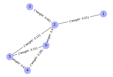
Poniższym poleceniem tworzony jest graf losowy Wattsa-Strogatza o dziesięciu węzłach (n = 10), o średniej ilości połączeń między wezłami równej 5 (k = 5), prawdopodobieństwie przełączenia danego wiązania równym 0.1 (rewire_prob = 0.1), początkowej liczbie agentów dysponujących informacją równej 10% populacji (initiation_perc = 0.1). Dodatkowo funkcja wyświetla atrybuty węzłów wraz z wagami (show_attr = True), oraz tworzy graf (draw_graph = True).

    Input:

G, pos = dp.graph_init(n = 10, 
                       k= 5,
                       rewire_prob = 0.1, 
                       initiation_perc = 0.1,
                       show_attr = True, 
                       draw_graph = True)

    Output:

Node attributes:
0 {'state': 'unaware', 'receptiveness': 1.0, 'extraversion': 0.582378, 'engagement': 1e-06}
1 {'state': 'unaware', 'receptiveness': 0.800181, 'extraversion': 0.329359, 'engagement': 0.028751}
2 {'state': 'unaware', 'receptiveness': 0.385395, 'extraversion': 0.226138, 'engagement': 0.623113}
3 {'state': 'aware', 'receptiveness': 0.368734, 'extraversion': 0.14079, 'engagement': 0.398072}
4 {'state': 'unaware', 'receptiveness': 0.306774, 'extraversion': 0.244501, 'engagement': 0.023409}
5 {'state': 'unaware', 'receptiveness': 0.275711, 'extraversion': 0.879711, 'engagement': 0.275111}
6 {'state': 'unaware', 'receptiveness': 0.578056, 'extraversion': 0.308108, 'engagement': 0.786855}
7 {'state': 'unaware', 'receptiveness': 0.844748, 'extraversion': 1e-06, 'engagement': 0.838986}
8 {'state': 'unaware', 'receptiveness': 0.702168, 'extraversion': 0.578449, 'engagement': 0.294877}
9 {'state': 'unaware', 'receptiveness': 0.807228, 'extraversion': 0.808263, 'engagement': 0.866605}
Wages:
0 [1.e-06]
1 [0.012265]
2 [0.020133]
3 [0.046409]
4 [0.053141]
5 [0.089238]
6 [0.094578]
7 [0.095085]
8 [0.23072]
9 [0.245545]
10 [0.271505]
11 [0.29906]
12 [0.310618]
13 [0.38126]
14 [0.397444]
15 [0.467515]
16 [0.512404]
17 [0.591285]
18 [0.641824]
19 [1.]

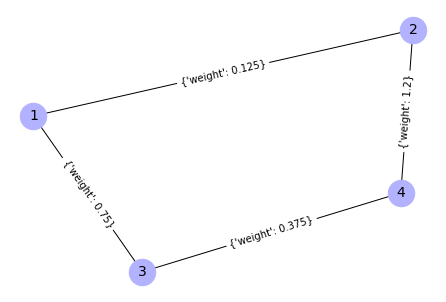
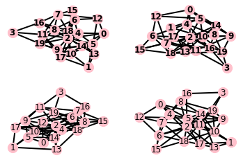
W ramach działania funkcji automatycznie generowane są dla grafu losowe wagi, losowane z rozkładu wykładniczego i oznaczają prawdopodobieństwa kontaktu między poszczególnymi agentami. Przypisywane są one do krawędzi grafu, czyli odpowiadają relacjom między węzłami. Dodatkowo generowane są cztery atrybuty przypisane do węzłów. Są to kolejno receptiveness – receptywność, extraversion – ekstrawersja, engagement – zaangażowanie, state – stan węzła. Poziom receptywności jest losowany z rozkładu normalnego i oznacza zdolność agenta do odbierania bodźców ze środowiska. Poziom ekstrawersji jest również generowany z rozkładu normalnego i odpowiada poziomowi ekstrawersji agenta w psychologicznej koncepcji klasyfikacji osobowości Carla G. Junga. Zaangażowanie oznacza poziom zaangażowania aktora w dany temat, na ile jest on związany swoim doświadczeniem z tematem w którego zakresie leży informacja. Zaangażowanie jest losowane z rozkładu wykładniczego. Wszystkie trzy atrybuty ilościowe są skalowane do przedziału (0,1] w celu ułatwienia przeprowadzenia symulacji, która odwołuje się później do tych wartości. Stan węzła jest atrybutem dwupoziomowym i przyjmuje wartość aware – świadomy i unaware – nieświadomy w kontekście posiadania danej informacji. Powyższe cechy służą później do dobliczania szansy na przeniesienie się informacji między poszczególnymi węzłami. Szansa ta jest obliczana dla każdej relacji między węzłami w jądrze symulacji nazwanym “WERE” zaimplementowanym w module simulate.py. Nazwa “WERE” to akronim od nazw parametrów biorących udział w obliczeniach. Pakiet umożliwia wykorzystanie dowolnego własnego równania, zamieniając jądro “WERE” na własną funkcję.

draw_graph()

Funkcja draw_graph() odpowiedzialna jest za wizualizację grafu. Może być wywoływana z poziomu funkcji graph_init(), z argumentem draw_graph == True. Funkcja draw_graph() odwołuje się do biblioteki NetworkX z funkcjami draw_networkx_nodes(), draw_networkx_labels(), draw_networkx_edges(), które z kolei bazują na bibliotece Matplotlib. Funkcja przyjmuje pięć argumentów:

1) G – obiekt grafowy biblioteki NetworkX, ze zdefiniowaną zmienną state przypisaną do węzłów,
2) pos – zmienna typu ndarray, która przechowuje pozycje węzłów grafu niezbędne do wizualizacji,
3) aware_color – zmienna typu string, która określa kolor węzłów świadomych danej informacji, przyjmuja wartości określające kolor w zapisie Hex
4) not_aware_color – zmienna typu string, która określa kolor węzłów nieświadomych danej informacji,
5) legend – zmienna typu bool, która odpowiada za dodanie legendy do wykresu.

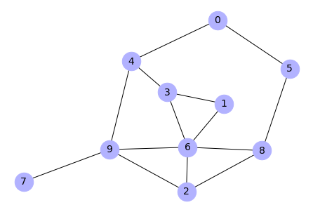
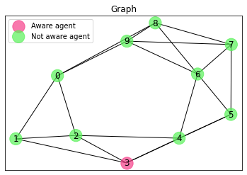
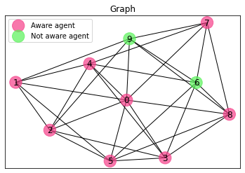
Aby wykorzystać tę funkcję, niezbędny jest atrybut state przypisany do węzłów grafu, z wartościami aware i unaware określającymi, które węzły są w posiadaniu informacji. Funkcja wyświetla wykres grafu.

    Input:

dp.draw_graph(G, # graph
              pos, # position of nodes
              aware_color = '#f63f89',
              not_aware_color = '#58f258',
              legend = True)

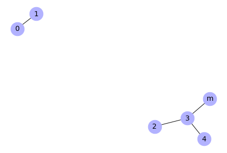
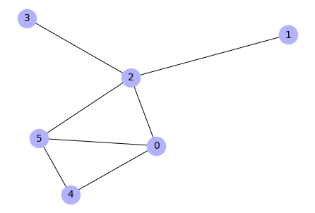
    Output:

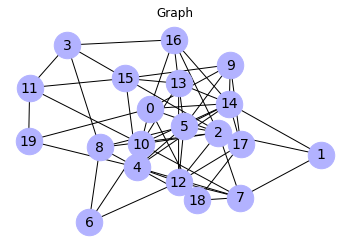
graph_stats()

Funkcja graph_stats() służy do obliczania podstawowych statystyk grafu. Funkcja przyjmuje pięć argumentów:

1) G – obiekt klasy grafu biblioteki NetworkX,
2) pos – zmienna typu ndarray, która przechowuje pozycje węzłów grafu niezbędne do wizualizacji,
3) show_attr – typ bool, umożliwia wyświetlenie wag i atrybutów węzłów danego grafu,
4) draw_degree – typ bool, określenie wartości jako True odpowiada za utworzenie wykresu rozkładu stopni węzłów grafu,
5) draw_graph – typ bool, umożliwia utworzenie wykresu grafu.

Funkcja zwraca obiekt dict_stat – typu słownikowego, zawierający podstawowe statystyki grafu, takie jak liczbę węzłów sieci, liczbę krawędzi, wagi połączeń między węzłami, atrybuty węzłów.

    Input:

dp.graph_stats(G,
		pos,
		show_attr = False,
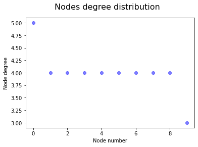
		draw_degree = True, 
		draw_graph = False)

    Output:

General information:

nodes :  10
edges :  20
mean node degree :  4
average clustering coefficient :  0.4833
transitivity :  0.4918

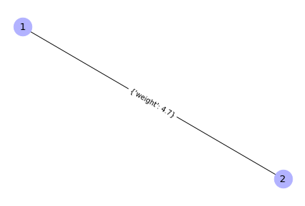
add_feature()

Funkcja add_feature() odpowiada za dodanie atrybutów do grafu z opcjonalnym skalowaniem tych atrybutów do przedziału (0,1]. Wywołując funkcję graph_init() zmienne są przyporządkowywane do węzłów automatycznie, natomiast funkcja add_feature() daje większą kontrolę nad dodawaną zmienną. Funkcja przyjmuje osiem argumentów:

1) G – obiekt klasy grafu biblioteki NetworkX,
2) pos – zmienna typu ndarray, która przechowuje pozycje węzłów grafu niezbędne do wizualizacji,
3) feature – zmienna typu ndarray, będąca atrybutem przypisywanym do węzłów grafu,
4) feature_type – zmienna typu string, mająca poziomy: “weights”, “receptiveness”, “extraversion”, “engagement”, “state”, lub inne dowolne nazwy,
5) scaling – typ bool, argument opcjonalny, umożliwia skalowanie dodanej zmiennej do przedziału (0,1],
6) decimals – typ integer, argument opcjonalny, odpowiada za liczbę cyfr po przecinku przy zaokrąglaniu,
7) show_attr – typ bool, umożliwia wyświetlenie wag i atrybutów węzłów danego grafu,
8) draw_graph – typ bool, argument opcjonalny, odpowiada za utworzenie wykresu grafu.
Funkcja zwraca zmienną G – graf, który jest obiektem klasy grafu NetworkX.

    Input:

import networkx as nx

# Create basic watts-strogatz graph
G_02 = nx.watts_strogatz_graph(n = 10, k = 6, p = 0.3, seed=None)

# Compute a position of graph elements
pos = nx.spring_layout(G_02)

import numpy as np

# Create example weights
weights = np.round(np.random.exponential(scale = 0.1, 
	size = G_02.number_of_edges()), 6).reshape(G_02.number_of_edges(),1)

# Add feature
G_02 = dp.add_feature(G_02,
                   pos,
                   feature = weights,
                   feature_type = "weights",
                   scaling = True,
                   decimals = 6,
                   show_attr = True, # show node weights and attributes
                   draw_graph = False)

    Output:

Nodes' attributes:

0 {}
1 {}
2 {}
3 {}
4 {}
5 {}
6 {}
7 {}
8 {}
9 {}

Sorted weights:

0 1e-06
1 0.010339
2 0.01119
3 0.038441
4 0.049669
5 0.051154
6 0.068371
7 0.081067
8 0.082919
9 0.086678
10 0.110474
11 0.121775
12 0.12913
13 0.132083
14 0.152151
15 0.164671
16 0.182431
17 0.187515
18 0.245855
19 0.268703
20 0.339081
21 0.407199
22 0.545156
23 0.560313
24 0.654668
25 0.683216
26 0.713856
27 0.770032
28 0.98711
29 1.0

    Input:

# Create example engagement
engagement = np.round(np.random.exponential(scale = 0.1, 
size = G_02.number_of_edges()), 6).reshape(G_02.number_of_edges(),1)

# Add feature
G_02 = dp.add_feature(G_02,
		pos,
		feature = engagement,
		feature_type = "engagement",
		scaling = True,
		show_attr = True, # show node weights and attributes
		draw_graph = False)

    Output:

Nodes' attributes:

0 {'engagement': 0.28056}
1 {'engagement': 0.196385}
2 {'engagement': 0.001351}
3 {'engagement': 1.0}
4 {'engagement': 0.187343}
5 {'engagement': 0.004473}
6 {'engagement': 0.305583}
7 {'engagement': 0.10013}
8 {'engagement': 0.113332}
9 {'engagement': 0.031052}

Sorted weights:

0 1e-06
1 0.010339
2 0.01119
3 0.038441
4 0.049669
5 0.051154
6 0.068371
7 0.081067
8 0.082919
9 0.086678
10 0.110474
11 0.121775
12 0.12913
13 0.132083
14 0.152151
15 0.164671
16 0.182431
17 0.187515
18 0.245855
19 0.268703
20 0.339081
21 0.407199
22 0.545156
23 0.560313
24 0.654668
25 0.683216
26 0.713856
27 0.770032
28 0.98711
29 1.0

add_state_random()

Funkcja add_state_random() odpowiada za wygenerowanie zmiennej określającej czy dany aktor w sieci jest świadomy określonej informacji. Funkcja przyjmuje pięć parametrów:

1) G – obiekt grafowy biblioteki NetworkX,
2) pos – typ ndarray, przechowuje pozycje węzłów grafu niezbędne do wizualizacji,
3) initiation_perc – typ float, określa odsetek węzłów dysponujących początkowo informacją,
4) show_attr – typ bool, odpowiada za wyświetlenie wag i atrybutów węzłów danego grafu,
5) draw_graph – typ bool, opcjonalna, umożliwia utworzenie wykresu grafu.
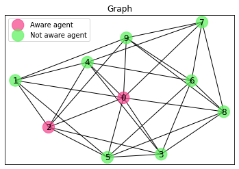
Funkcja zwraca zmienną G – obiekt klasy grafu NetworkX.

    Input:

# add state
dp.add_state_random(G_02, 
                    pos,
                    initiation_perc = 0.2, 
                    show_attr = True, 
                    draw_graph = True)

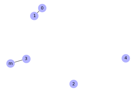
    Output:

Node attributes:
0 {'engagement': 0.28056, 'state': 'aware'}
1 {'engagement': 0.196385, 'state': 'unaware'}
2 {'engagement': 0.001351, 'state': 'aware'}
3 {'engagement': 1.0, 'state': 'unaware'}
4 {'engagement': 0.187343, 'state': 'unaware'}
5 {'engagement': 0.004473, 'state': 'unaware'}
6 {'engagement': 0.305583, 'state': 'unaware'}
7 {'engagement': 0.10013, 'state': 'unaware'}
8 {'engagement': 0.113332, 'state': 'unaware'}
9 {'engagement': 0.031052, 'state': 'unaware'}

2. Moduł symulacyjny

Moduł simulate.py służy do przeprowadzenia symulacji rozchodzenia się informacji w sieciach. Składa się z funkcji simulation_step(), simulation() i simulation_sequence(). W module simulate.py istnieje możliwość wykorzystania funkcji simulation_step() do generowania pojedynczych kroków symulacji. Na każdym kroku symulacji można tworzyć wykres bieżącej struktury sieci. Funkcja simulation() do symulacji wielokrokowych wywołuje funkcję simulation_step() i dodaje nowe funkcjonalności udostępniając parametry funkcji simulation_step() oraz dodatkowy parametr liczby przeprowadzonych symulacji. Analogicznie działa funkcja simulation_sequence() do sekwencji symulacji wielokrokowych, która opakowuje funkcję simulation() i udostępnia również dodatkowe parametry. Taka struktura umożliwia wykorzystanie funkcji simulation_step() jako podstawy symulacji i dopisywanie własnych dodatkowych elementów kodu w razie potrzeby. W funkcji simulation_sequence() zaimplementowano metodę Monte Carlo. Wykorzystano ją do obliczania zdolności propagacji informacji zadanego zestawu węzłów. Element mechanizmu losowego przeszukiwania zaszyty jest w funkcji simulation_step(), w której proces symulacyjny jest oparty o zmienne losowe, wyrażające prawdopodobieństwa kontaktu między węzłami w sieci.

simulation_step()

Funkcja simulation_step() wykonuje jeden krok symulacji i nadpisuje zmiany parametrów w grafie. Przyjmuje osiem argumentów:

1) G – obiekt klasy grafu biblioteki NetworkX,
2) pos – przyjmuje zmienną typu ndarray, która przechowuje pozycje węzłów grafu niezbędne do wizualizacji.
3) kernel – typ string, posiada poziomy “weights”, “WERE” i “custom”. Parametr określony jako “weights” aplikuje do symulacji jądro, które podczas rozprzestrzeniania się informacji bierze pod uwagę tylko wagi na krawędziach między węzłami. Po ustawieniu parametru jako “WERE” – do obliczania prawdopodobieństwa przekazania informacji między węzłami jest aplikowane równanie oparte na parametrach weights-extraversion-receptiveness-engagement przyporządkowanych do węzłów sieci. Aby uruchomić symulację z tym jądrem, graf powinien mieć zdefiniowane powyższe zmienne, przypisane do wierzchołków grafu. Natomiast z wartością “custom” – prawdopodobieństwo rozchodzenia się informacji jest obliczane z własną zdefiniowaną funkcją,
4) Engagement_enforcement – typ float, liczba podana jako argument jest mnożnikiem parametru engagement dla poszczególnych węzłów, które są już świadome, lub zapomniały informację po danej iteracji,
5) custom_kernel – dowolna funkcja obliczająca prawdopodobieństwo przekazania informacji w każdym kroku symulacji dla każdego węzła. Funkcja może operować na zmiennych przypisanych do wierzchołków grafu,
6) WERE_multiplier – typ float, argument opcjonalny, odpowiada za regulację wartości obliczanej przez jądro “WERE”,
7) oblivion – typ bool, argument opcjonalny, odpowiada za zapominanie agentów o informacji.
8) draw – typ bool, argument opcjonalny, umożliwia utworzenie wykresu grafu.

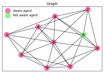
Funkcja zwraca zmienną G – graf, który jest obiektem klasy grafu NetworkX. Poniżej przeprowadzone są dwa kroki symulacji na grafie zaprezentowanym powyżej, podczas omawiania funkcji add_state_random() .

    Input:

# Copy graph 
import copy
G_03 = copy.deepcopy(G_02)

# Perform one simulation step
G_03 = dp.simulation_step(G_03, 
                       pos,
                       kernel = 'weights', 
                       custom_kernel = None,
                       WERE_multiplier = 10, 
                       oblivion = False, 
                       engagement_enforcement = 1.01,
                       draw = True, 
                       show_attr = False)

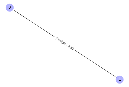
    Output:

    Input:

# Perform one simulation step
G_03 = dp.simulation_step(G_03, 
                       pos,
                       kernel = 'weights', 
                       custom_kernel = None,
                       WERE_multiplier = 10, 
                       oblivion = False, 
                       engagement_enforcement = 1.01,
                       draw = True, 
                       show_attr = False)

    Output:

simulation()

Funkcja simulation() wykonuje zadaną liczbę kroków symulacji i zwraca graf z nadpisanymi parametrami. Funkcja przyjmuje dziewięć argumentów – osiem argumentów zapożyczonych z funkcji simulation_step(), oraz dodatkowy argument n o typie integer, określający liczbę kroków w symulacji. Funkcja zwraca następujące zmienne:

1) G – graf, który jest obiektem klasy grafu NetworkX,
2) graph_list, zmienną typu lista przechowującą informacje o stanie węzłów we wszystkich krokach sytuacji. Lista składa się wewnętrznych list. Każda wewnętrzna lista odnosi się do odpowiadającego jej kroku w symulacji.
3) avg_aware_inc_per_step – lista przechowująca średni przyrost świadomych agentów na jeden krok symulacji.

    Input:

# Copy graph 
G_03 = copy.deepcopy(G_02)

# Simulation
graph_list, avg_aware_inc_per_step \
= dp.simulation(G_03, 
               pos,
               n = 2,
                      
               kernel = 'weights', 
               custom_kernel = None,
               WERE_multiplier = 10, 
               oblivion = False, 
               engagement_enforcement = 1.01,
               draw = False, 
               show_attr = False)
    
print(avg_aware_inc_per_step)

import pprint
pprint.pprint(graph_list)

    Output:

3.5

[[(0, {'engagement': 0.28056, 'state': 'aware'}),
  (1, {'engagement': 0.196385, 'state': 'unaware'}),
  (2, {'engagement': 0.001351, 'state': 'aware'}),
  (3, {'engagement': 1.0, 'state': 'unaware'}),
  (4, {'engagement': 0.187343, 'state': 'unaware'}),
  (5, {'engagement': 0.004473, 'state': 'unaware'}),
  (6, {'engagement': 0.305583, 'state': 'unaware'}),
  (7, {'engagement': 0.10013, 'state': 'unaware'}),
  (8, {'engagement': 0.113332, 'state': 'unaware'}),
  (9, {'engagement': 0.031052, 'state': 'unaware'})],
 [(0, {'engagement': 0.291953, 'state': 'aware'}),
  (1, {'engagement': 0.202335, 'state': 'aware'}),
  (2, {'engagement': 0.001407, 'state': 'aware'}),
  (3, {'engagement': 1.0, 'state': 'unaware'}),
  (4, {'engagement': 0.187343, 'state': 'unaware'}),
  (5, {'engagement': 0.004518, 'state': 'aware'}),
  (6, {'engagement': 0.305583, 'state': 'unaware'}),
  (7, {'engagement': 0.10013, 'state': 'unaware'}),
  (8, {'engagement': 0.113332, 'state': 'unaware'}),
  (9, {'engagement': 0.031363, 'state': 'aware'})],
 [(0, {'engagement': 0.309914, 'state': 'aware'}),
  (1, {'engagement': 0.210551, 'state': 'aware'}),
  (2, {'engagement': 0.001478, 'state': 'aware'}),
  (3, {'engagement': 1.040604, 'state': 'aware'}),
  (4, {'engagement': 0.187343, 'state': 'unaware'}),
  (5, {'engagement': 0.004796, 'state': 'aware'}),
  (6, {'engagement': 0.314842, 'state': 'aware'}),
  (7, {'engagement': 0.10013, 'state': 'aware'}),
  (8, {'engagement': 0.11561, 'state': 'aware'}),
  (9, {'engagement': 0.032963, 'state': 'aware'})]]

simulation_sequence()

Funkcja simulation_sequence() wykonuje sekwencję symulacji. Przekazuje ona argumenty do funkcji simulation(), oraz pobiera dodatkowy argument sequence_len o typie integer, określający liczbę symulacji w sekwencji. Funkcja zwraca zmienną avg_aware_inc typu float, która zawiera średni przyrost świadomych agentów na jeden krok dla wszystkich symulacji. Funkcja nie zwraca zmodyfikowanego grafu.

    Input:

avg_aware_inc_per_step = \
dp.simulation_sequence(G_03, # networkX graph object
                        #pos, # p
                        n = 2, # number of steps in simulation
                        sequence_len = 1000, # sequence of simulations
                              
                        kernel = 'weights', # kernel type
                        custom_kernel = None, # custom kernel function
                        WERE_multiplier = 10, 
                        oblivion = False, # information oblivion feature 
                        engagement_enforcement = 1.01,
                        show_attr = False)

    Output:

3.6325

3. Moduł optymalizacyjny

Celem działania funkcji z modułu optymalizacyjnego jest wyznaczenie n węzłów sieci, które najszybciej rozpropagują informację. W skład modułu wchodzi funkcja optimize_centrality() pozwalająca na obliczanie zestawu n węzłów cechujących się największym poziomem bliskości (ang. closeness) w sieci w stosunku do innych węzłów. Drugą funkcją jest optimize_rs(), która poszukuje najlepszych wierzchołków symulacyjnie za pomocą metody przeszukiwania losowego.

optimize_centrality()

Funkcja optimize_centrality() przyjmuje następujące argumenty:

1) G – graf, który jest obiektem klasy grafu NetworkX,
2) number_of_nodes – typ integer, oznacza liczbę węzłów do wytypowania.

Kolejna dwa argumenty przekazywane są do funkcji wyliczającej miarę bliskości węzłów z biblioteki NetworkX:

3) distance – typ string, parametr opcjonalny, wskazuje na nazwę atrybutu krawędzi, która ma zostać użyta do optymalizacji,
4) wf_improved – typ bool, argument przyjmuje wartość logiczną określającą użycie ulepszonej wersji algorytmu wyliczającego bliskość.

Funkcja zwraca obiekt n_best_nodes będący listą krotek, gdzie każda krotka zawiera numer węzła oraz jego miarę centralności. Do aproksymacji centralności węzła została zastosowana funkcja obliczająca bliskość (ang. closeness) między wierzchołkami grafu.

    Input:

# Copy graph 
G_03 = copy.deepcopy(G_02)


# Run function with weights as distances
dp.optimize_centrality(G_03,
                    distance = 'weight',
                    wf_improved = False,
                    number_of_nodes = 4)

    Output:

[(0, 13.02914620004951),
 (4, 13.02914620004951),
 (1, 13.029033028598729),
 (2, 9.811242593874512)]

optimize_rs()

Funkcja optimize_rs() przyjmuje osiem parametrów, które przekazuje do funkcji simulation_sequence:

1) G – obiekt klasy grafu biblioteki NetworkX,
2) n – typ integer; odpowiedzialny za liczbę kroków w symulacji,
3) sequence_len – parametr typu integer określający liczbę symulacji w jednej sekwencji,
4) kernel – typ string, posiada poziomy “weights”, “WERE” i “custom”, 5) custom_kernel – dowolna funkcja obliczająca prawdopodobieństwo przekazania informacji w każdym kroku symulacji dla każdego węzła. Funkcja może operować na zmiennych przypisanych do wierzchołków grafu,
6) WERE_multiplier – typ float, argument opcjonalny, odpowiada za regulację wartości obliczanej przez jądro “WERE”,
7) oblivion – typ bool, argument opcjonalny, odpowiada za zapominanie agentów o informacji.
8) Engagement_enforcement – typ float, liczba podana jako argument jest mnożnikiem parametru engagement dla poszczególnych węzłów,

oraz parametry:

9) number_of_nodes – typ integer, określa liczbę węzłów do wytypowania,
10) number_of_iter – typ integer, wyznacza liczbę iteracji w optymalizacji random search,
11) log_info_interval – typ integer, parametr opcjonalny, odpowiada za interwał iteracji pomiędzy kolejnymi wyświetleniami w konsoli informacji o postępie optymalizacji. Wartość ustawiona jako None ukrywa wyświetlanie informacji.

    Input:

solution = dp.optimize_rs(G_03,
        number_of_nodes = 2, # number of nodes to seed
        number_of_iter = 1000, # number of iterations 
        log_info_interval = 1, # interval of information log 
                       
        n = 3, # number of simulation steps simulation
        sequence_len = 100, # number of simulations in one seq
                       
        kernel = 'weights', # kernel type
        custom_kernel = None, # custom kernel function
        WERE_multiplier = 10, 
        oblivion = False, # information oblivion feature 
        engagement_enforcement = 1.00
        )
					   

    Output:

2 Iterations passed with best solution: 2.62 in 1.19 seconds.
3 Iterations passed with best solution: 2.62 in 1.59 seconds.
4 Iterations passed with best solution: 2.62 in 1.94 seconds.
5 Iterations passed with best solution: 2.62 in 2.38 seconds.
6 Iterations passed with best solution: 2.62 in 2.77 seconds.
7 Iterations passed with best solution: 2.6567 in 3.27 seconds.
8 Iterations passed with best solution: 2.6567 in 3.6 seconds.
9 Iterations passed with best solution: 2.6567 in 4.02 seconds.
10 Iterations passed with best solution: 2.6567 in 4.44 seconds.
.
.
995 Iterations passed with best solution: 2.6667 in 462.58 seconds.
996 Iterations passed with best solution: 2.6667 in 463.31 seconds.
997 Iterations passed with best solution: 2.6667 in 463.79 seconds.
998 Iterations passed with best solution: 2.6667 in 464.45 seconds.
999 Iterations passed with best solution: 2.6667 in 465.16 seconds.

Best aware agents increment per simulation step: 2.6666666666666634

Set of initial aware nodes: [4, 1]

4. Moduł modelująco-wyjaśniający

Celem działania modułu modelująco-wyjaśniającego jest rozpoznanie, które atrybuty węzłów sieci implikują zdolność tych węzłów do efektywnego rozprowadzania informacji. W tym celu niezbędne jest utworzenie zbioru danych, w którym określimy jak efektywnie poszczególne węzły rozprowadzają informację. Może to odbyć się na drodze przeprowadzania symulacji i sprawdzania zdolności dla każdego węzła (lub próby tych węzłów), lub na drodze obliczania miar centralności. Kiedy przeprowadzone zostaną wymagane obliczenia, utworzona zostanie nowa zmienna, która będzie zmienną wyjaśnianą w modelu. Natomiast zmiennymi wyjaśniającymi będą pozostałe atrybuty przyporządkowane do węzłów sieci. Po utworzeniu modelu matematycznego na takim zbiorze danych należy wykorzystać jedną z technik analitycznych umożliwiających rozpoznanie istotności, czy też wkładu poszczególnych zmiennych w wyjaśnianie zmienności wariancji zmiennej zależnej. W module zastosowano funkcję XGBRegressor() z biblioteki XGBoost, która modeluje dane. Następnie na modelu stosowana jest metoda feature_importances_() obliczająca istotność zmiennych w modelu. Po wyliczanej istotności można ocenić, które zmienne dotyczące węzłów mogą być wskaźnikami zdolności do szybkiej propagacji informacji po sieci. Tego typu zabieg dostarcza informacji jakie cechy węzłów są istotne z biznesowego punktu widzenia. Przekładając to na przykładowy problem biznesowy – dowiemy się jakimi kryteriami powinien posłużyć się decydent, aby wybrać influencera do swojej kampanii marketingowej.

Moduł zawiera dwie funkcje: nodes_score_simulation() służącą do obliczenia miary nośności informacji dla każdego węzła, oraz feature_importance() odpowiadającą za obliczanie związku innych atrybutów węzłów z metryką wyliczoną przez nodes_score_simulation().

nodes_score_simulation()

Funkcja nodes_score_simulation() odpowiada za obliczenie średniego przyrostu świadomych agentów w sieci na jeden krok symulacji dla każdego węzła jako początkowego seedera. Funkcja przyjmuje dziewięć parametrów:

1) log_info_interval – typ integer, parametr opcjonalny, odpowiada za interwał iteracji pomiędzy kolejnymi wyświetleniami w konsoli informacji o postępie w obliczaniu miary centralności dla węzłów. Ustawiona wartość jako None ukrywa wyświetlanie informacji.

Osiem pozostałych parametrów przekazywanych jest kolejno do funkcji simulation_sequence(), oraz do bardziej zagnieżdżonych funkcji simulation() i simulation_step, i są to kolejno:

2) G – graf biblioteki NetworkX,
3) sequence_len – parametr typu integer określający liczbę symulacji w jednej sekwencji,
4) n – typ integer; odpowiedzialny za liczbę kroków w symulacji,
5) kernel – typ string, nazwa jądra symulacji, posiada poziomy “weights”, “WERE” i “custom”,
6) engagement_enforcement – typ float, liczba podana jako argument jest mnożnikiem parametru engagement dla poszczególnych węzłów, którę są już świadome, lub zapomniały informację po danej iteracji,
7) custom_kernel – dowolna funkcja obliczająca prawdopodobieństwo przekazania informacji w każdym kroku symulacji dla każdego węzła,
8) WERE_multiplier – typ float, argument opcjonalny, odpowiada za regulację wartości obliczanej przez jądro WERE,
9) oblivion – typ bool; opcjonalny; umożliwia włączenie opcji zapominania informacji przez agentów.

Funkcja zwraca obiekt list_solution będący listą z obliczonymi miarami szybkości propagacji informacji dla pojedynczych węzłów. Każda wartość to średni przyrost świadomych węzłów w sieci na jeden krok symulacji.

    Input:

solution = dp.nodes_score_simulation(G_03, 
                       log_info_interval = 1, # interval of information log 
                       
                       n = 3, # number of simulation steps simulation
                       sequence_len = 100, # number of simulations in one seq
                       
                       kernel = 'weights', # kernel type
                       custom_kernel = None, # custom kernel function
                       WERE_multiplier = 10, 
                       oblivion = False, # information oblivion feature 
                       engagement_enforcement = 1.00
                       )

    Output:

1 Iterations passed in 0.89 seconds.
2 Iterations passed in 1.28 seconds.
3 Iterations passed in 1.66 seconds.
4 Iterations passed in 2.0 seconds.
5 Iterations passed in 2.35 seconds.
6 Iterations passed in 2.71 seconds.
7 Iterations passed in 3.0 seconds.
8 Iterations passed in 3.31 seconds.
9 Iterations passed in 3.54 seconds.

List of solutions: [2.7766666666666664, 2.783333333333333, 
2.9166666666666656, 2.833333333333333, 2.733333333333333, 
2.7666666666666657, 2.7200000000000006, 2.453333333333333, 
2.6166666666666663, 2.1999999999999993]

feature_importance()

Funkcja feature_importance() służy do obliczania związku pomiędzy zmienną przechowującą miary węzłów, a innymi zmiennym przypisanymi do węzłów.
Funkcja przyjmuje 11 argumentów, z czego 9 argumentów jest identycznych z oczekiwanymi w funkcji nodes_score_simulation() i są one do niej przekazywane. Pozostałe dwa argumenty to:
1) X – typ ndarray, przyjmuje dwuwymiarową tablicę ze zmiennymi, których związek będzie sprawdzany ze zmienną zwróconą przez funkcję nodes_score_simulation(),
2) show – typ bool, odpowiada za wyświetlenie wyników w konsoli po zakończeniu działania funkcji.

Poniżej do zmiennej Y przypisano obliczone miary nośności informacji dla węzłów grafu G_03 wykorzystywanego w przykładach powyżej. Utworzono również 3 sztuczne zmienne skorelowane ze zmienną X w celu przetestowania funkcji feature_importance().

    Input:

import numpy as np
import math
from scipy.linalg import toeplitz, cholesky
from statsmodels.stats.moment_helpers import cov2corr

#=======================================#
# Create theoretical correlation matrix #
#=======================================#
p = 4 # total number of variables
h = 2/p
# create vector as a base for our next correlation matrix
v = np.linspace(1,-1+h,p)
# Create theoretical correlation matrix
R = cov2corr(toeplitz(v))

#===========================#
# create the first variable # (our "given variable")
# ==========================#
Y = solution

#=================================#
# generate p-1 correlated randoms #
#=================================#
# Generate 4 random variables
X_01 = np.random.randn(len(G_03),p)
# In 1 column insert our existing variable
X_01[:,0] = Y
# Cholesky decomposition (create some kind of matrix)
C = cholesky(R)
# Matrix product of two arrays. (iloczyn macierzowy)
X = np.matmul(X_01,C)


# set 6 digit decimal
np.set_printoptions(precision=6)
np.set_printoptions(suppress=True)

# remove 1st column (target variable)
X = np.delete(X, 0, 1)


FI = dp.feature_importance(
                       G_03, # NetworkX graph
                       X, # Nodes attributes 
                       show = True,
                       log_info_interval = 10, # interval of information log 
                       
                       n = 3, # number of simulation steps simulation
                       sequence_len = 20, # number of simulations in one seq
                       
                       kernel = 'weights', # kernel type
                       custom_kernel = None, # custom kernel function
                       WERE_multiplier = 10, 
                       oblivion = False, # information oblivion feature 
                       engagement_enforcement = 1.00
                       )

    Output:

List of solutions: [2.95, 2.9166666666666665, 2.8333333333333335, 
2.8166666666666664, 2.7333333333333334, 2.833333333333333, 
2.7666666666666666, 2.65, 2.6666666666666665, 1.85]

Feature importances:

Variable 1 : 0.8862867
Variable 2 : 0.03555947
Variable 3 : 0.07815386

Annotation

Satellites Tracking in Python

#python   #satellites   #n2yo REST API   #space industry

Sojuz-TMA on orbit, source: NASA

Space industry is the one of the most exciting fields of data science application areas. Data related to space we may get from radio telescopes, sky cameras, or devices installed on satellites, such as cameras, and other sensors. One type of data is a location of satellites itself. While the sky is clear, it is even possible to spot some of them with a naked eye, especially while phenomenon like satellite flare occurs – one may see satellite passing through the sky with enhanced flash during a few seconds.

Satellites and another objects on the Earth orbit are catalogued in Satellite Catalog Number, known also as NORAD Catalog Number. NORAD means North American Aerospace Defense Command - organisation incorporating United States and Canada. Its purpose is to provide aerospace warning and air sovereignty for North America.

For satellites tracking we may use N2YO.COM REST API. Detailed instructions are available at https://www.n2yo.com/api/. The current limit is 1000 transactions per hour. According to official documentation we may use the API to provide data for software/web applications involving satellite tracking or predicting their locations. In Terms of Use section, we may discover the main source of data:

The software used for tracking is using mainly space surveillance data provided by “Space Track”, a website consisting of a partial catalog of observations collected by the US Space Surveillance Network, operated by US Air Force Space Command (AFSPC). AFSPC does not make any warranties as to the accuracy or completeness of the data provided (…)

“Space Track” website has a limit of 200 requests per hour. So n2yo probably gets the data from space track, implement its own algorithms to predict information about satellites, and redistribute it for 5 times higher API requests limit for wider audience.

It is not the only one source of data. As we may see:

In special circumstances for a few satellites the traking data (“keplerian elements”) are derived from public sources (monitoring or visual observation)

but there is not specified what sources are they exactly, and for which satellites. Let’s look at main data source again. On space-track.org we may read that:

As the United States government agency responsible for Space Situational Awareness (SSA) information, United States Space Command (USSPACECOM), is committed to promoting a safe, stable, sustainable, and secure space environment through SSA information sharing. As more countries, companies, and non-governmental organizations field space capabilities and benefit from the use of space systems, it is in our collective interest to act responsibly and to enhance overall spaceflight safety. To achieve effective SSA, USSPACECOM seeks to increase cooperation and collaboration with partners and space-faring entities through the exchange of SSA data and provision of SSA services.

This means that USSPACECOM encurages institutions to cooperation and releases data. Information about space objects are available via API after estabilishing user account, but advanced access requires custom Orbital Data Request, or SSA Sharing Agreement. What may be interesting for polish readers, according to official website of Polish Space Agency - polsa.gov.pl, POLSA has signed such an agreement on April 10, 2019 with USSTRATCOM for sharing SSA information (USSPACECOM was merged with USSTRATCOM at the time and was not independent entity).

N2YO.COM API offers a few methods to get information about satellites. Below four methods are described, without “Get radio passes” method, which may be useful, when someone want to estabilish a direct connection with satellites, for example with Software Defined Radio. Due to presentation clarity some of the output responses below code snippets will be shown.

Contents:
1. TLE method,
2. Positions method,
3. Visualpasses method,
4. Above method.

1. TLE method

TLE method is responsible for getting TLE - “Two-line element set”. TLE is special data format which encodes information about certain object on the planet orbit, such as NORAD Catalog Number, satellite number, satellite classification, satellite launch year, launch number of the year, and more.

To communicate with API we will use get method from requests package. To get apiKey necessary to estabilish connection we need to register an account at n2yo.com, and after login visit the profile page and push the button that creates the API key.

# Import requests library 
import requests

# Define satellite NORAD Catalog Number of choosen satellite
sat_id_01 = '13242'

# Define API KEY (your API key from n2yo.com)
apiKey = 'R4BXQP-LPVRES-2TJMDS-33P2'

# Use get method
r_01 = requests.get(url = "https://www.n2yo.com/rest/v1/satellite/tle/" \
	+ sat_id_01 + "&apiKey=" + apiKey) 

# Check response code, if response == 200, request was performed correctly
r_01

    Output:

<Response [200]>

Data extraction

# Extract data in JSON format 
data_01 = r_01.json() 

# Print obtained data
import json
print(json.dumps(data_01, indent = 2))

    Output:

{
  "info": {
    "satid": 13242,
    "satname": "SL-8 R/B",
    "transactionscount": 2
  },
  "tle": "1 13242U 82051B   20075.75668091 +.00000023 +00000-0 
  +16967-4 0 9992\r\n2 13242 074.0438 313.4556 0025991 267.9974 
  091.8203 14.35970955977236"
}

We may see above that response variable is just a dictionary, so we extract data with its keys.

# Extract Satellite name
data_01['info']['satname']

# Extract transactions count in last 60 minutes
data_01['info']['transactionscount']

# Extract "2-line" TLE informations
data_01['tle']

    Output:

'1 13242U 82051B   20075.75668091 +.00000023 +00000-0 +16967-4 0  
9992\r\n2 13242 074.0438 313.4556 0025991 267.9974 091.8203 
14.35970955977236'

2. Positions method

This method is used to predict future positions of given satellite. Request returns satellite’s latitude, longitude as independent coordinates, and azimuth, elevation with respect to the observer location.

Response array contains number of elements set by “seconds” parameter. If “seconds” parameter is set to ‘2’, as a result we get an array with first element for current UTC time, and second element for current UTC time + 1 second. If we set this parameter to ‘3’ we will get an array with data for current UTC time, current UTC time + 1 second, and current UTC time + 2 seconds, etc.

At first we need to set parameters of the request

# Satellite id (there in an example for International Space Station)
sat_id_02 = '25544'

There we set location parameters for Warsaw, Poland

# Observer's latitide in decimal degrees
lat_02 = '52.237049'

# Observer's longitude in decimal degrees
lng_02 = '21.017532'

# Observer's altitude above sea level in meters
alt_02 = '100'

# Number of satellite positions to return 
#(each position for each further second with limit 300 seconds)
sec_02 = '2' # return positions for current time, and current time + 1 second

Send a request

r_02 = requests.get(url = "https://www.n2yo.com/rest/v1/satellite/positions/" 
                 + sat_id_02+ '/' + lat_02 + '/' + lng_02 + '/' + alt_02 + '/' 
                 + sec_02 + '/' + "&apiKey=" + apiKey) 

# Check request message
r_02

    Output:

<Response [200]>

Extract data

# Extract data in JSON format 
data_02 = r_02.json() 

# Print obtained data
import json
print(json.dumps(data_02, indent = 2))

    Output:

{
  "info": {
    "satname": "SPACE STATION",
    "satid": 25544,
    "transactionscount": 0
  },
  "positions": [
    {
      "satlatitude": 19.04015824,
      "satlongitude": 99.09844139,
      "sataltitude": 421.38,
      "azimuth": 87.08,
      "elevation": -31.16,
      "ra": 283.11435926,
      "dec": -22.47502746,
      "timestamp": 1584397228
    },
    {
      "satlatitude": 18.9911662,
      "satlongitude": 99.13901737,
      "sataltitude": 421.38,
      "azimuth": 87.08,
      "elevation": -31.19,
      "ra": 283.1412382,
      "dec": -22.50212702,
      "timestamp": 1584397229
    }
  ]
}

# Show data with key "info"
data_02['info']

# Show NORAD Catalog Number used in input
data_02['info']['satid']

# Satellite name
data_02['info']['satname']

# Count of transactions in last 60 minutes for present API key
data_02['info']['transactionscount']

Show coordinates of satellite in present time

# Satellite footprint latitude in decimal degrees
data_02['positions'][0]['satlatitude']

# Satellite footprint longitude in decimal degrees
data_02['positions'][0]['satlongitude']

# Satellite footprint altitude in kilometers
data_02['positions'][0]['sataltitude']

## Location with respect to the observer

# Satellite azimuth with respect to observer's location in degrees
data_02['positions'][0]['azimuth']

# Satellite elevation with respect to observer's location in degrees
data_02['positions'][0]['elevation']

## Location with respect to the earth 

# Satellite right ascension in degrees
data_02['positions'][0]['ra']

# Satellite declination in degrees
data_02['positions'][0]['dec']

# Get Unix timestamp in seconds for this position
data_02['positions'][0]['timestamp']

# Convert Unix timestamp value to observer's UTC time 
from datetime import datetime
print(datetime.fromtimestamp(data_02['positions'][0]['timestamp']).strftime('%Y-%m-%d %H:%M:%S'))

    Output:

1584397228
2020-03-16 23:20:28

To show coordinates of satellite in present time + 1 second, we need to relate to second element of a list with [1] instead of [0].

3. Visualpasses method

Visualpasses method is used to get information about consecutive visual passes of choosen satellite indicated by NORAD Catalog Number, from given place on the earth. To spot the satellite it should be above the horizon, illuminated, and the sky should be dark enough. Firstly, to perform the query, we need to set request parameters such as observer’s coordinates.

Parameters setting

# Satellite id (there is International Space Station as an example)
sat_id_03 = '25544'

# Observer's latitide in decimal degrees (for Warsaw)
lat_03 = '52.237049'

# Observer's longitude in decimal degrees
lng_03 = '21.017532'

# Observer's altitude above sea level in meters
alt_03 = '100'

# Number of days of prediction (max 10)
days_03 = '5'

# Minimal time of satellite visibility in seconds to be considered 
# in the request
min_visibility_03 = '5'

Send a request

r_03 = requests.get(url = "https://www.n2yo.com/rest/v1/satellite/visualpasses/" 
                 + sat_id_03+ '/' + lat_03 + '/' + lng_03 + '/' + alt_03 + '/' 
                 + days_03 + '/' + min_visibility_03 + "&apiKey=" + apiKey) 

# Check request message
r_03

    Output:

<Response [200]>

Data extraction

# Extract data in JSON format 
data_03 = r_03.json() 

# Print obtained data
print(json.dumps(data_03, indent = 2))

    Output:

{
  "info": {
    "satid": 25544,
    "satname": "SPACE STATION",
    "transactionscount": 1,
    "passescount": 4
  },
  "passes": [
    {
      "startAz": 197.46,
      "startAzCompass": "SSW",
      "startEl": 0.02,
      "startUTC": 1584640715,
      "maxAz": 140.58,
      "maxAzCompass": "SE",
      "maxEl": 13.02,
      "maxUTC": 1584640985,
      "endAz": 82.75,
      "endAzCompass": "E",
      "endEl": 12.83,
      "endUTC": 1584641255,
      "mag": 0.1,
      "duration": 250
    },
    {
      "startAz": 228.93,
      "startAzCompass": "SW",
      "startEl": 0.08,
      "startUTC": 1584729990,
      "maxAz": 152.23,
      "maxAzCompass": "SSE",
      "maxEl": 34.07,
      "maxUTC": 1584730305,
      "endAz": 78.4,
      "endAzCompass": "E",
      "endEl": 27.74,
      "endUTC": 1584730610,
      "mag": -0.9,
      "duration": 255
    },
    {
      "startAz": 219.26,
      "startAzCompass": "SW",
      "startEl": 0.06,
      "startUTC": 1584813545,
      "maxAz": 148.7,
      "maxAzCompass": "SE",
      "maxEl": 25.27,
      "maxUTC": 1584813850,
      "endAz": 78.71,
      "endAzCompass": "E",
      "endEl": 19.46,
      "endUTC": 1584814150,
      "mag": -0.8,
      "duration": 385
    },
    {
      "startAz": 253.27,
      "startAzCompass": "WSW",
      "startEl": 0.13,
      "startUTC": 1584819315,
      "maxAz": 162.78,
      "maxAzCompass": "SSE",
      "maxEl": 69.02,
      "maxUTC": 1584819640,
      "endAz": 82.8,
      "endAzCompass": "E",
      "endEl": 20.33,
      "endUTC": 1584819955,
      "mag": -0.4,
      "duration": 195
    }
  ]
}

# Show general information about passes
data_03['info']

    Output:

{'satid': 25544,
 'satname': 'SPACE STATION',
 'transactionscount': 1,
 'passescount': 4}

First pass

# Satellite azimuth for the start of this pass 
# (relative to the observer, in degrees)
data_03['passes'][0]['startAz']

# Satellite elevation for the start of this pass 
# (relative to the observer, in degrees)
data_03['passes'][0]['startEl']

# get Unix timestamp for the start of this pass 
data_03['passes'][0]['startUTC']

# convert Unix timestamp value to observer's UTC time 
from datetime import datetime
print(datetime.fromtimestamp(data_03['passes'][0]['startUTC']).strftime('%Y-%m-%d %H:%M:%S'))

    Output:

1584640715
2020-03-19 18:58:35

# Satellite azimuth for the max elevation of this pass 
# (relative to the observer, in degrees)
data_03['passes'][0]['maxAz']

# Satellite max elevation for this pass 
# (relative to the observer, in degrees)
data_03['passes'][0]['maxEl']

# Unix time for the max elevation of this pass. 
# We should convert this UTC value to observer's time zone
data_03['passes'][0]['maxUTC']

# Max visual magnitude of the pass, same scale as star brightness. 
# If magnitude cannot be determined, the value is 100000
data_03['passes'][0]['mag']

# Total visible duration of this pass in seconds
data_03['passes'][0]['duration']

To show the second (and further) satellite pass if predicted, we need to relate to second element of the list with [1] instead of [0].

4. Above method

This method is used to get the information about objects in given radius related to the observer. Radius parameter is expressed in range from 0 to 90 degrees. If radius is larger, more space for search is used. This is very interesting method for people who want to spot some satellites during the night from certain place on the earth.

Parameters setting

# Observer's latitide in decimal degrees (for Warsaw)
observer_lat_05 = '52.237049'

# Observer's longitude in decimal degrees
observer_lng_05 = '21.017532'

# Observer's altitude above sea level in meters
observer_alt_05 = '100'

# Search radius (range from 0 to 90)
search_radius_05 = '3'

# Category id 
category_id_05 = '0'
# Category id == 0 means search in all categories

Send a request

r_05 = requests.get(url = "https://www.n2yo.com/rest/v1/satellite/above/" 
                 + observer_lat_05 + '/' + observer_lng_05 + '/' 
                 + observer_alt_05 + '/' + search_radius_05 + '/' 
                 + category_id_05 + "&apiKey=" + apiKey) 

# Check request message
r_05

    Output:

<Response [200]>

Data extraction

# Extracting data in JSON format 
data_05 = r_05.json() 

# Print obtained data
import json
print(json.dumps(data_05, indent = 2))

    Output:

{
  "info": {
    "category": "ANY",
    "transactionscount": 0,
    "satcount": 2
  },
  "above": [
    {
      "satid": 36549,
      "satname": "COSMOS 2251 DEB",
      "intDesignator": "1993-036BDK",
      "launchDate": "1993-06-16",
      "satlat": 50.4823,
      "satlng": 23.4983,
      "satalt": 5.2306528291122e+19
    },
    {
      "satid": 38203,
      "satname": "COSMOS 2251 DEB",
      "intDesignator": "1993-036BST",
      "launchDate": "1993-06-16",
      "satlat": 51.9402,
      "satlng": 22.982,
      "satalt": 6.0611831651699e+16
    }
  ]
}

# Category name (ANY if category id requested was 0)
data_05['info']['category']

# Count of transactions performed with this API key in last 60 minutes
data_05['info']['transactionscount']

# Count of satellites returned
data_05['info']['satcount']

# Satellite NORAD Catalog Number
data_05['above'][0]['satid']

# Satellite name
data_05['above'][0]['satname']

# Satellite launch date (YYYY-MM-DD)
data_05['above'][0]['launchDate']

# Satellite footprint latitude in decimal degrees
data_05['above'][0]['satlat']

# Satellite footprint longitude in decimal degrees
data_05['above'][0]['satlng']

# Satellite altitude in kilometers
data_05['above'][0]['satalt']

To sum up, we described shortly and ilustrated usage of four methods to identify location of satellites used in n2yo REST API: TLE method, positions method, visualpasses method, and above method. There is also one more method called radiopasses, which may be used to get information about passes of certain satellites with which radio contact is possible from a given place on the earth.

Annotation

Social Network Analysis in Python - Introduction to NetworkX

#python   #networkx   #social network analysis

NetworkX is a Python library for working with graphs and perform analysis on them. It has built-in many fancy features like algorithms for creating specific graphs genres, or some centrality measures. But in this article we concentrate on work at grassroots - how to create graph, add and remove nodes and edges, add weighted edges, inspect graph properties an visualize graphs.

“By definition, a Graph is a collection of nodes (vertices) along with identified pairs of nodes (called edges, links, etc). In NetworkX, nodes can be any hashable object e.g., a text string, an image, an XML object, another Graph, a customized node object, etc.”
— NetworkX documentation

Content below is based on very good NetworkX documentation where you can go deeper into NetworkX. In this post you may see simple examples how to use code.

Contents:
1. Create a graph
2. Add nodes, edges, weighted edges to a graph
3. Add attributes to graphs, nodes, edges
4. Check a graph properties
5. Access edges and neighbors
6. Draw graphs
7. Graphs I/O in GML format

1. Create a graph

Create an empty graph

# Import library
import networkx as nx

# Create an empty graph - collection of nodes
G = nx.Graph()

# Create a directed graph using connections from the previous graph G
H = nx.DiGraph(G)

# Clear the graph from all nodes and edges 
# it deletes also graph attributes, nodes attributes and edges attributes.
G.clear()

Create a graph from list of edges

# Create a list of edges (list of tuples)
edgelist = [(0, 1), (1, 2), (2, 3)]

# Create a graph
H = nx.Graph(edgelist)

# Draw a graph
%matplotlib inline

# Draw a plot
nx.draw(H, with_labels=True, node_color='#b2b2ff', node_size=700, 
	font_size=14)

    Output:

Create a graph from an adjacency matrix

# Create an adjacency matrix
import numpy as np
adj_m = np.array([[0, 1, 1],
                  [1, 1, 1],
                  [0, 1, 0]])

# Create a graph
G = nx.from_numpy_matrix(adj_m)

# Draw the graph
nx.draw(G, with_labels=True, node_color='#b2b2ff', node_size=700, 
	font_size=14)

    Output:

Create a chain graph

# Create a chain graph (5 nodes from 0 to 4)
H = nx.path_graph(5)

# Draw the graph
nx.draw(H, with_labels=True, node_color='#b2b2ff', node_size=700, 
	font_size=14)

    Output:

2. Add nodes, edges, weighted edges to a graph

Add nodes to a graph

# Create an empty graph
G = nx.Graph()

# Add a node 
G.add_node(1)

# Draw the graph
nx.draw(G, with_labels=True, node_color='#b2b2ff', node_size=700, 
	font_size=14)

    Output:

# Add a list of nodes
G.add_nodes_from([2, 3])

# Draw the graph
nx.draw(G, with_labels=True, node_color='#b2b2ff', node_size=700, 
	font_size=14)

    Output:

# Create a chain graph (5 nodes from 0 to 4)
H = nx.path_graph(5)
# Show created nodes
H.nodes

    Output:

NodeView((0, 1, 2, 3, 4))

# Add nodes from the graph H to the graph G (nodes 1,2,3 are overwrited)
G.add_nodes_from(H)
G.nodes

    Output:

NodeView((1, 2, 3, 0, 4))

We can see above that numbers play role of something like keys of particular nodes in graph. And this nodes may be overwritten.

# Draw the graph
nx.draw(G, with_labels=True, node_color='#b2b2ff', node_size=700, 
	font_size=14)

    Output:

# Add a node as a string label
G.add_node("la") # adds node "la"
G.nodes

    Output:

NodeView((1, 2, 3, 0, 4, 'la'))

# Add nodes as single string elements
G.add_nodes_from("la")  # adds 2 nodes: 'l', 'a'
G.nodes

    Output:

NodeView((1, 2, 3, 0, 4, 'la', 'l', 'a'))

Remove nodes from the graph

# Remove a node
G.remove_node(2)

# Draw the graph
nx.draw(G, with_labels=True, node_color='#b2b2ff', node_size=700, 
	font_size=14)

    Output:

# Remove nodes from an iterable container
G.remove_nodes_from([3,4])

# Draw the graph
nx.draw(G, with_labels=True, node_color='#b2b2ff', node_size=700, 
	font_size=14)

    Output:

Add edges to a graph

# Create an empty graph
G = nx.Graph()

# Add an edge between node 1 and node 2
G.add_edge(1, 2)

# Draw the graph
nx.draw(G, with_labels=True, node_color='#b2b2ff', node_size=700, 
	font_size=14)

    Output:

We can see above that if an edge is created - all needed non-existing nodes are created as well.

# Create a tuple with 2, 3
e = (2, 3)
type(e)

    Output:

tuple

# Use the tuple to create an edge between nodes 2 and 3
G.add_edge(*e)
G.edges

    Output:

EdgeView([(1, 2), (2, 3)])

# Draw the graph
nx.draw(G, with_labels=True, node_color='#b2b2ff', node_size=700, 
	font_size=14)

    Output:

# Create a chain graph (5 nodes from 0 to 4)
H = nx.path_graph(5)
# Add edges to graph G from graph H
G.add_edges_from(H.edges)
G.edges

    Output:

EdgeView([(1, 2), (1, 0), (2, 3), (3, 4)])

# Draw the graph
nx.draw(G, with_labels=True, node_color='#b2b2ff', node_size=700, 
	font_size=14)

    Output:

# Add an edge between node 3 and non-existing node m - which is automatically
#                                                                  created
G.add_edge(3, 'm')

# Draw the graph
nx.draw(G, with_labels=True, node_color='#b2b2ff', node_size=700, 
	font_size=14)

    Output:

Remove edges from a graph

# Remove an edge
G.remove_edge(1, 2)

# Draw the graph
nx.draw(G, with_labels=True, node_color='#b2b2ff', node_size=700, 
	font_size=14)

    Output:

# Remove edges from an iterable container
G.remove_edges_from([(2, 3),(3,4)])

# Draw the graph
nx.draw(G, with_labels=True, node_color='#b2b2ff', node_size=700, 
	font_size=14)

    Output:

Add weighted edges to a graph

# Create an empty graph
G = nx.Graph()

# Add an edge with weight as a tuple with a dictionary inside on a 3rd position  
G.add_edge(0, 1, weight=2.8)

G.edges

    Output:

EdgeView([(0, 1)])

# Compute a position of the graph elements (needed to visualize weighted graphs)
pos = nx.spring_layout(G)
# Draw the graph
nx.draw(G, pos = pos, with_labels=True, node_color='#b2b2ff', node_size=700, 
	font_size=14)
# Add weights to the graph picture
nx.draw_networkx_edge_labels(G, pos)

    Output:

{(0, 1): Text(0.0, 0.0, "{'weight': 2.8}")}

    Output:

Create Erdős-Rényi graph

For an example we use Erdős-Rényi graph generation. It takes only one short line of code. This is a simple and powerful way of creating graphs. Method “erdos_renyi_graph()” takes 2 arguments. 1st is number of nodes, and second one is probability that a node will get an edge connection with every other particular node. So if more nodes, probability of node having any edge rise.

# Import library
import random
import numpy as np

# Generate Erdos-renyi graph 
G = nx.gnp_random_graph(6,0.4) # (gnp alias from: G-raph, N-odes, 
                               #                    P-robability)
nx.draw(G, with_labels=True, node_color='#b2b2ff', node_size=700, 
	font_size=14)

    Output:

Add random weights to the graph

# add random weights 
for u,v,d in G.edges(data=True):
    d['weight'] = round(random.random(),2) # there we may set distribution
    # in this loop we iterate over a tuples in a list
    #                    u - is actually 1st node of an edge
    #                    v - is second node of an edge
    #                    d - is dict with weight of edge

# Extract tuples of adges, and weights from the graph
edges,weights = zip(*nx.get_edge_attributes(G,'weight').items())
print(weights, edges)

# Compute a position of graph elements (needed to visualize weighted graphs)
pos = nx.spring_layout(G)
# draw graph
nx.draw(G, pos = pos, with_labels=True, node_color='#b2b2ff', node_size=700, 
	font_size=14)
# Add weights to graph picture
nx.draw_networkx_edge_labels(G, pos)

    Output:

(0.67, 0.28, 0.31, 0.61, 0.66, 0.13, 0.63) ((0, 2), (0, 4), (0, 5), (1, 2), (2, 3), (2, 5), (4, 5))

    Output:

{(0, 2): Text(0.05587924164442272, 0.03572413385076614, "{'weight': 0.67}"),
 (0, 4): Text(-0.09144909073877293, -0.6331454386897136, "{'weight': 0.28}"),
 (0, 5): Text(-0.18708205101864206, -0.43166771273736326, "{'weight': 0.31}"),
 (1, 2): Text(0.36606551732176823, 0.4975472153877831, "{'weight': 0.61}"),
 (2, 3): Text(-0.03165513391993038, 0.6029900698900599, "{'weight': 0.66}"),
 (2, 5): Text(-0.14019660265009343, -0.12965270150716987, "{'weight': 0.13}"),
 (4, 5): Text(-0.2875249350332891, -0.7985222740476496, "{'weight': 0.63}")}

    Output:

Note that positions of nodes may differ from the unweighted graph, but structure of the graph is the same

3. Add attributes to a graph, nodes and edges

Add attributes to a graph

# Create a graph
G = nx.Graph()
# Add 'day' attribute to the graph with "Friday" value
G = nx.Graph(day = "Friday")
G.graph

    Output:

{'day': 'Friday'}

# Change an attribute value
G.graph['day'] = "Monday"
G.graph

    Output:

{'day': 'Monday'}

# Delete graph attribute
del G.graph['day']

G.graph

    Output:

{}

Add attributes to nodes

# Create a graph
G = nx.Graph()

# Add an attribute "time" with value, for node 1
G.add_node(1, time='5pm')

# Add the attribute "time" with value, for node 3
G.add_nodes_from([3], time='2pm')

# Check attributes of 1 node
G.nodes[1]

    Output:

{'time': '5pm'}

# Check attributes of 3 node
G.nodes[3]

    Output:

{'time': '2pm'}

# Add an attribute "room" with value, for node 1
G.nodes[1]['room'] = 714
G.nodes.data()

    Output:

NodeDataView({1: {'time': '5pm', 'room': 714}, 3: {'time': '2pm'}})

# delete particular node attribute
del G.nodes[1]['room']

# Print nodes attributes
G.nodes.data()

    Output:

NodeDataView({1: {'time': '5pm'}, 3: {'time': '2pm'}})

# Print nodes attributes
for k, v in G.nodes.items():
    print(f'{k:<4} {v}')

    Output:

1    {'time': '5pm'}
3    {'time': '2pm'}

# Delete 'time' attributes from all nodes in a loop
for k, v in G.nodes.items():
    del G.nodes[k]['time']

# Print node attributes
for k, v in G.nodes.items():
    print(f'{k:<4} {v}')

    Output:

1    {}
3    {}

Add attributes to an edges

# Create a graph
G = nx.Graph()

# Add weighted edge to graph    
G.add_edge(1, 2, weight=4.7 )

# Compute position of the graph elements
pos = nx.spring_layout(G)
# Draw the graph
nx.draw(G, pos = pos, with_labels=True, node_color='#b2b2ff', node_size=700, 
	font_size=14)
# Add weights to a graph picture
nx.draw_networkx_edge_labels(G, pos)

    Output:

{(1, 2): Text(2.220446049250313e-16, 0.0, "{'weight': 4.7}")}

    Output:

Weights are one type of attributes. We may create custom attributes.

# Add 2 edges with attribute color to the graph     
G.add_edges_from([(2, 3), (3, 4)], color='red')

# Compute a position of graph elements
pos = nx.spring_layout(G)
# Draw the graph
nx.draw(G, pos = pos, with_labels=True, node_color='#b2b2ff', node_size=700, 
	font_size=14)
# Add attributes to graph picture
nx.draw_networkx_edge_labels(G, pos)

    Output:

{(1, 2): Text(-0.6545391148791944, 0.17485675574125337, "{'weight': 4.7}"),
 (2, 3): Text(-0.07544906355289227, 0.020149585725262716, "{'color': 'red'}"),
 (3, 4): Text(0.6545391148791944, -0.17485675574125328, "{'color': 'red'}")}

    Output:

# Another way to add an attribute
G.add_edges_from([(1, 2, {'color': 'blue'}), (2, 3, {'weight': 8})])

# Another way to add an attribute
G.edges[1,2]['color'] = "white"
# Check added properties of edges
G.adj.items()

    Output:

ItemsView(AdjacencyView({1: {2: {'weight': 4.7, 'color': 'white'}}, 2: {1: {'weight': 4.7, 'color': 'white'}, 3: {'color': 'red', 'weight': 8}}, 3: {2: {'color': 'red', 'weight': 8}, 4: {'color': 'red'}}, 4: {3: {'color': 'red'}}}))

# Print edges attributes in more readable way 
for k, v, w in G.edges.data():
    print(f'{k:<4} {v}{w}')

    Output:

1    2{'weight': 4.7, 'color': 'white'}
2    3{'color': 'red', 'weight': 8}
3    4{'color': 'red'}

In the printings above we can see that node 1 has connection with node 2. And this edge has attributes weight and color. Node 2 has 2 connections - with node 1 and node 3.

# Add a weight for an edge 1-2
G[1][2]['weight'] = 4.7

# or
G.edges[1, 2]['weight'] = 4.7    

# Check attributes on edges
G.edges.data()

    Output:

EdgeDataView([(1, 2, {'weight': 4.7, 'color': 'white'}), (2, 3, {'color': 'red', 'weight': 8}), (3, 4, {'color': 'red'})])

# Print edges attributes in more readable way 
for k, v, w in G.edges.data():
    print(f'{k:<4} {v}{w}')

    Output:

1    2{'weight': 4.7, 'color': 'white'}
2    3{'color': 'red', 'weight': 8}
3    4{'color': 'red'}

# Delete edge attribute 
del G[2][3]['color']

# Print edges attributes 
for k, v, w in G.edges.data():
    print(f'{k:<4} {v}{w}')

    Output:

1    2{'weight': 4.7, 'color': 'white'}
2    3{'weight': 8}
3    4{'color': 'red'}

G.edges.data()

    Output:

EdgeDataView([(1, 2, {'weight': 4.7, 'color': 'white'}), (2, 3, {'weight': 8}), (3, 4, {'color': 'red'})])

# Delete edge attributes "weight"
for n1, n2, d in G.edges(data=True):
    if "weight" in d:
        del d["weight"]

# Print edges attributes 
for k, v, w in G.edges.data():
    print(f'{k:<4} {v}{w}')

    Output:

1    2{'color': 'white'}
2    3{}
3    4{'color': 'red'}

4. Check a graph properties

Prepare a graph

# Create a chain graph
G = nx.path_graph(5)
# Draw the graph
nx.draw(G, with_labels=True, node_color='#b2b2ff', node_size=700, 
	font_size=14)

    Output:

Check properties

# Check number of nodes
G.number_of_nodes()

    Output:

5

# Check number of edges
G.number_of_edges()

    Output:

4

Nodes View

# All nodes overview
G.nodes()

    Output:

NodeView((0, 1, 2, 3, 4))

# or
list(G.nodes)

    Output:

[0, 1, 2, 3, 4]

# or
G.nodes.items()

    Output:

ItemsView(NodeView((0, 1, 2, 3, 4)))

# or
G.nodes.data()

    Output:

NodeDataView({0: {}, 1: {}, 2: {}, 3: {}, 4: {}})

# or
G.nodes.data('span')

    Output:

NodeDataView({0: None, 1: None, 2: None, 3: None, 4: None}, data='span')

Edges View

# All edges overview
G.edges

    Output:

EdgeView([(0, 1), (1, 2), (2, 3), (3, 4)])

# or
list(G.edges)

    Output:

[(0, 1), (1, 2), (2, 3), (3, 4)]

# or
G.edges.items()

    Output:

ItemsView(EdgeView([(0, 1), (1, 2), (2, 3), (3, 4)]))

# or (weights visible)
G.edges.data()

    Output:

EdgeDataView([(0, 1, {}), (1, 2, {}), (2, 3, {}), (3, 4, {})])

# or (weights visible)
G.edges.data('span')

    Output:

EdgeDataView([(0, 1, None), (1, 2, None), (2, 3, None), (3, 4, None)])

# or (for an iterable container of nodes) - all edges associated with this 
#                                                       subset of nodes
G.edges([2, 'm'])

    Output:

EdgeDataView([(2, 1), (2, 3)])

Node degree View

# Check degree of particular nodes
G.degree

    Output:

DegreeView({0: 1, 1: 2, 2: 2, 3: 2, 4: 1})

# list degrees in column (":<4" makes 4 spaces between numbers)
for v, d in G.degree():
    print(f'{v:<4} {d}')

    Output:

0    1
1    2
2    2
3    2
4    1

# or (for the one particular node)
G.degree[1]

    Output:

2

# or (for the iterable container of nodes)
G.degree([2, 3])

    Output:

DegreeView({2: 2, 3: 2})

Adjacency view

# Check an adjacency matrix - neighbourhood between nodes
G.adj

    Output:

AdjacencyView({0: {1: {}}, 1: {0: {}, 2: {}}, 2: {1: {}, 3: {}}, 3: {2: {}, 4: {}}, 4: {3: {}}})

# Print a dictionary in a dictionary in more readable way 
from pprint import pprint
pprint(dict(G.adj))

    Output:

{0: AtlasView({1: {}}),
 1: AtlasView({0: {}, 2: {}}),
 2: AtlasView({1: {}, 3: {}}),
 3: AtlasView({2: {}, 4: {}}),
 4: AtlasView({3: {}})}

# Check neighbors of particular node
list(G.adj[3])

    Output:

[2, 4]

# or
G[3]

    Output:

AtlasView({2: {}, 4: {}})

# or
list(G.neighbors(3))

    Output:

[2, 4]

5. Accessing edges and neighbors

# Create a graph
G = nx.Graph()
G.add_weighted_edges_from([(1, 2, 0.125), (1, 3, 0.75), (2, 4, 1.2), 
                           (3, 4, 0.375)])

# Compute position of graph elements
pos = nx.spring_layout(G)
# Draw the graph
nx.draw(G, pos = pos, with_labels=True, node_color='#b2b2ff', node_size=700, 
	font_size=14)
# Add weights to a graph picture
nx.draw_networkx_edge_labels(G, pos)

    Output:

{(1, 2): Text(-0.11306457583748142, 0.3689242447964494, "{'weight': 0.125}"),
 (1, 3): Text(-0.7453632597697203, -0.1911266592810591, "{'weight': 0.75}"),
 (2, 4): Text(0.74536325976972, 0.19112665928105907, "{'weight': 1.2}"),
 (3, 4): Text(0.11306457583748117, -0.3689242447964495, "{'weight': 0.375}")}

    Output:

1st method for edges + weights extraction

# Get 'weight' attributes
nx.get_edge_attributes(G,'weight').items()

    Output:

dict_items([((1, 2), 0.125), ((1, 3), 0.75), ((2, 4), 1.2), ((3, 4), 0.375)])

# Build up variables
edges,weights = zip(*nx.get_edge_attributes(G,'weight').items())

# Edges overview
edges # tuple of tuples

    Output:

((1, 2), (1, 3), (2, 4), (3, 4))

# Weights overview
weights # tuple

    Output:

(0.125, 0.75, 1.2, 0.375)

2nd method for edges + weights extraction

for (u, v, wt) in G.edges.data('weight'):
    print('(%d, %d, %.3f)' % (u, v, wt))

    Output:

(1, 2, 0.125)
(1, 3, 0.750)
(2, 4, 1.200)
(3, 4, 0.375)

2nd method for edges + weights extraction with condition

for (u, v, wt) in G.edges.data('weight'):
    if wt < 0.5: print('(%d, %d, %.3f)' % (u, v, wt))

    Output:

(1, 2, 0.125)
(3, 4, 0.375)

6. Draw graphs

Figure size changing

# Import libraries
import networkx as nx
import matplotlib.pyplot as plt

# Graph creation
G = nx.erdos_renyi_graph(20, 0.30)

# Draw a graph
plt.figure(1) # default figure size 
plt.title("Graph") # Add title
nx.draw(G, with_labels=True, node_color='#b2b2ff', node_size=700, 
	font_size=14)

# Draw a big graph
plt.figure(2,figsize=(10,10)) # Custom figure size
plt.title("Big Graph") # Add title
nx.draw(G, with_labels=True, node_color='#b2b2ff', node_size=700, 
	font_size=14)

    Output:

    Output:

Draw 2 graphs on 1 chart

# Create graph
G = nx.erdos_renyi_graph(20, 0.20)

# Draw graphs with "nx.draw" and subplots 
# Nr 121, 122 are for 2 graphs on 1 chartplt.subplot(121)

# Draw graph 1
plt.subplot(121)
plt.title("Graph 1")
nx.draw(G, with_labels=True, node_color='#b2b2ff', node_size=700, 
	font_size=14)

# Draw graph 2
plt.subplot(122)
plt.title("Graph 2")
nx.draw(G, with_labels=True, node_color='#b2b2ff', node_size=700, 
	font_size=14)

    Output:

Draw 4 graphs on 1 chart with kwargs

In the situation where we have to define arguments for many subplots we may use “kwargs” (keyworded arguments) feature. It allows us to define a dictionary contains keys with values, which become arguments of a function. Clear explanation of this feature you may find there.

# Create graph
G = nx.erdos_renyi_graph(20, 0.30)

# Define **kwargs - dictionary with arguments for a function
kwargs = {
    'node_color': 'pink',
    'node_size': 200,
    'width': 2, # 
    }

# Draw graphs with options
# Nr 221, 222, 223, 224 are for 4 graphs on 1 chart
plt.subplot(221)
nx.draw(G, with_labels=True, font_weight='bold', **kwargs)
plt.subplot(222)
nx.draw(G, with_labels=True, font_weight='bold', **kwargs)
plt.subplot(223)
nx.draw(G, with_labels=True, **kwargs)
plt.subplot(224)
nx.draw(G, with_labels=True, **kwargs)

    Output:

Draw a graph with more arguments specified

plt.title("Graph")
nx.draw(G, # graph object 
        with_labels=True, # label of node (numbers of nodes in this case)
        node_size=500, 
        node_color="#ffcc99", 
        node_shape="o", 
        alpha=0.7, # node transparency
        linewidths=1, # linewidth of symbol borders (nodes)
        width=1, # linewidth of edges
        edge_color="purple", 
        style="dashed", # style of edges
        font_size=12, 
        fontcolor="k", 
        font_family="Consolas")

    Output:

• with_labels (bool, optional (default=True)) – Set to True to draw labels on the nodes.
  
• node_size (scalar or array, optional (default=300)) – Size of nodes. If an array is specified it must be the same length as nodelist
  
• node_color (color string, or array of floats, (default=’#1f78b4’)) – Node color. Can be a single color format string, or a sequence of colors with the same length as nodelist. If numeric values are specified they will be mapped to colors using the cmap and vmin,vmax parameters. See matplotlib.scatter for more details.
  
• node_shape (string, optional (default=’o’)) – The shape of the node. Specification is as matplotlib.scatter marker, one of ‘so^>v<dph8’.
  
• alpha (float, optional (default=1.0)) – The node and edge transparency
  
• linewidths ([None | scalar | sequence]) – Line width of symbol border (default =1.0)
  
• width (float, optional (default=1.0)) – Line width of edges
  
• edge_color (color string, or array of floats (default=’r’)) – Edge color. Can be a single color format string, or a sequence of colors with the same length as edgelist. If numeric values are specified they will be mapped to colors using the edge_cmap and edge_vmin,edge_vmax parameters.
  
• style (string, optional (default=’solid’)) – Edge line style (solid|dashed|dotted,dashdot)
  
• font_size (int, optional (default=12)) – Font size for text labels
  
• font_color (string, optional (default=’k’ black)) – Font color string
  
• font_family (string, optional (default=’sans-serif’)) – Font family
  

Check more arguments in NetworkX documentation.

Add random weights to a graph and draw as colored edges

Very interesting way for visualize weighted graph is to color its edges depending on weights.

# Generate Erdős-Rényi graph
G = nx.gnp_random_graph(10,0.3)
nx.draw(G, with_labels=True, node_color='#b2b2ff', node_size=700, 
	font_size=14)

    Output:

# Add random weights 
for u,v,d in G.edges(data=True):
    d['weight'] = random.random() # there we may set distribution
    # in this loop we iterate over a tuples in a list
    #                    u - is actually 1st node of an edge
    #                    v - is second node of an edge
    #                    d - is dict with weight of edge
    
# Extract tuples of adges, and weights from the graph
edges,weights = zip(*nx.get_edge_attributes(G,'weight').items())

# Compute optimized nodes positions
pos = nx.spring_layout(G)
# Draw graph
nx.draw(G, pos, edgelist=edges, 
        edge_color=weights, width=3.0, edge_cmap=plt.cm.Blues, 
        edge_vmin=-0.4, edge_vmax=1, with_labels=True,
		node_color='#b2b2ff', node_size=700, font_size=14)

    Output:

Note that positions of nodes may differ from the unweighted graph, but structure of the graph is the same.

7. Graphs I/O in GML format

• write GML file nx.write_gml(graph, "path.to.file")

• read GML file mygraph = nx.read_gml("path.to.file")

Annotation

Python Virtual Environment - virtualenv

#python   #virtualenv   #devops

Sometimes there is a situation that one want to run some code found on the internet to automate some tasks. But programming language is been developing as well as libraries. So after time code found on the internet is outdated.

So there are two ways to deal with outdated code. We may rewrite it to the current version. The second way is to configure environment to the state, when the code was working well. Normally we may just reinstall some libraries to the desired versions typing pip reinstall 'module_name==desired_version', for example pip install 'xkcdpass==1.2.5' or pip install 'xkcdpass==1.2.5' --force-reinstall --ignore-installed. Unfortunately after many libraries reinstallations some errors may occurs.

In this article I will describe how to adjust environment in Anaconda to the specific version of Python interpreter and Python modules.

Contents:
1. Set up virtualenv on Windows 10,
2. Enabling Spyder,
3. Multiple Python versions handling.

1. Set up virtualenv on Windows 10

• Open Anaconda prompt

• Install library pip install virtualenv

• Go to particular catalog in Anaconda prompt cd C:\your\catalog\path

• Set up “venv” virtual environment with virtualenv library python -m virtualenv venv

• If virtual env was set up (some folders created in our catalog), we can activate environment venv\Scripts\activate. After activation of environment - “(venv)” shows up in the path in the command line.

• Now we have empty virtual environment. W may install packages with specific versions there pip install tale==3.4

• To save all versions of modules installed in our environment we may write “requirements.txt” file pip freeze > requirements.txt

• with requirements.txt we may reproduce state of our environment in any time by installing modules listed there pip install -r requirements.txt

• Deactivation of virtual environment deactivate

2. Enabling Spyder

Spyder installation

• To run Spyder we need to install required kernels in our activated virtual environment pip install spyder-kernels==0.*

• or install Spyder pip install spyder, but in this way virtual environment is heavy and has over 350 MB at the beginning

Run Spyder in virtual environment

• Run Spyder normally as before new installation

• Go to: Tools -> preferences -> Python interpreter -> Use the following Python interpreter

• Paste path of python.exe from virtual environment folder, apply changes and click Ok

• Restart console in Spyder by closing current console window. New console working with virtual environment should be loaded

3. Multiple Python versions handling

To create virtual environment on Windows 10 with certain Python version we may create Anaconda environment with specific Python version (if not exists yet). We may specify a catalog for installation, and Python version.

• When “python=3.6” specified, Anaconda with the latest version of Python 3.6 will be installed conda create --prefix C:/ProgramData/anaconda36 python=3.6

• After activation conda activate C:/ProgramData/anaconda36 subtitle “base” is changing on path given above in Anaconda prompt. On top of that we may build virtual environment

• virtualenv installation (coz new Anaconda virtualenv is clean of additional pkgs) pip install virtualenv

• Go to particular catalog in Anaconda prompt cd C:\path\to\catalog\where\you\want\virtualenv

• Set up “venv” virtual environment with Python version from particular Anaconda installation. We need specify path of Python interpreter from new Anaconda environment python -m virtualenv -p "C:\ProgramData\anaconda36\python.exe" venv

• Activation of virtual environment - venv\Scripts\activate

• Install required things to run Spyder pip install spyder-kernels==0.*. Now we can run Spyder and adjust its interpreter as before. After installation of modules in specified versions with pip install 'module_name==desired_version' we may run scripts which demand specified Python version, and specified modules versions

• Deactivation of virtual environment deactivate

• Dezactivation of anaconda environment conda deactivate

• Remove conda environment conda remove --name py36 --all

Annotation

Code Highlighting and Formatting Cheetsheet in Jekyll

#html   #markdown   #jekyll

Creating a blog demands using some amount of graphical motives. In this place formatting and graphical motives are aggregated, useful in creating visual aspect of a Jekyll website. To explore motives presented below go to github repository. to “_posts” catalog, and open this post to look at code behind that.

Contents:
1. Code highlighting,
2. Text formatting.

1. Code highlighting

Code highlighting in markdown

<a class="sidebar-nav-item" href="/blog"></a>

Code highlighting in markdown - python code snippet

class Singleton:
    def __new__(self):
        print("la")
        # check whether obcject (self) has attribute "instance"
        
        # if hasattr function is evaluated as FALSE (object self not have instance)
        if not hasattr(self, 'instance'):
            
            # new instance is created
            self.instance = super().__new__(self)
            # __new__ is a method which create new instance of class
            # super is a reference to parent class
            
        # if hasattr function is evaluated as TRUE, just return existing instance
        # (so no new instance will be created )
        return self.instance
        # so this line making that we will get the same object even if we want
        # to create next object
    
    def method_01(self):
        print("lala")

Code highlighting in markdown with raw clause

<a class="sidebar-nav-item{% if page.url == node.url %} 
active{% endif %}" href="{{site.baseurl}}{{ node.url }}">{{ node.title }}</a>

Code highlighting in markdown showing markdown code

``` html
<a class="sidebar-nav-item{% if page.url == node.url %} 
active{% endif %}" href="{{site.baseurl}}{{ node.url }}">{{ node.title }}</a>
```

Code highlighting in markdown - when language not recognized

print("Something")

Deprecation: You appear to have pagination turned on, but you haven't included the `jekyll-paginate` gem. Ensure you have `plugins: [jekyll-paginate]` in your configuration file.  

Rogue code highlighting in rectangle sharp frame

def print_hi(name)
  puts "Hi, #{name}"
end
print_hi('Tom')
#=> prints 'Hi, Tom' to STDOUT.

Rogue code highlighting with code numeration

1
2
3
def foo
  puts 'foo'
end

Some command line or small code snippets

Code

or

More code

Html code block

  
    puts "hello"
  

Embedding gist code

2. Text formatting

Div container - annotations

Border around text

First example with text surrounded by a colored border.
This example also has multiple lines.

Border around text with regulated width

First example with text surrounded by a colored border.
This example also has multiple lines.

Border around text with regulated width 2

First example with text surrounded by a colored border.
This example also has multiple lines.

Border around text with regulated width and text wrapped

First example with text surrounded by a colored border.
This example also has multiple lines.

Wrapped text. Wrapped text. Wrapped text. Wrapped text. Wrapped text. Wrapped text. Wrapped text. Wrapped text. Wrapped text. Wrapped text. Wrapped text. Wrapped text.

Text area

Text area 2

Inline font change

Dependency Error: Yikes! It looks like you don’t have jekyll-paginate or one of its dependencies installed.

Inline font change 2

Roses are red.

Markdown colored text

Some Markdown text with some blue text.

Markdown colored text in div container

Tekst with line on the left

Tekst with line
on the left

Bullet points

• One point
• second point

Special characters writing in html

{
%
}
 
`

Text bolding

bolded text

or

bolded text also

Italicization

italicized text

Italicization + align attribute

Source: NASA

Abbreviations

HTML

Citation

— Werner Heisenberg

Deletion

Deleted something

Insertion

inserted

Superscription

Something^text

Subscription

Something_text

Align attribute - text to left

This is some text in a paragraph.

Align attribute - text to center

This is some text in a paragraph.

Align attribute - text to right

This is some text in a paragraph.

Linebreak with specified size

Bulletpoints

• First bullet
• second
• third

Numeration

1. First number
2. second
3. third

External link type 1

link somewhere

External link type 2 (with opening in a new window)

link somewhere

Table

Table 2

Latex equations (mathjax)

Depending on the value of \(x\) the equation \(f(x) = \sum_{i=0}^{n} \frac{a_i}{1+x}\) may diverge or converge.

Source: overleaf.com

Photo uploading

Source: unsplash.com

Embedding Plotly chart-studio plot in iframe with plot centering

Embedding Shiny app plot in iframe with plot centering

Annotation